This project focusses on building the intuition needed for 2D convolutions and filtering and then learning how to use frequencies to sharpen images, combine two images into one and blend two images using multiresolution blending.
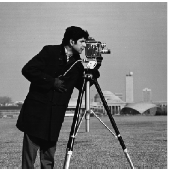
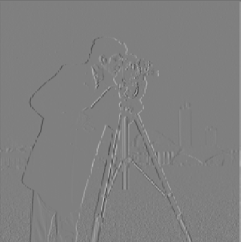
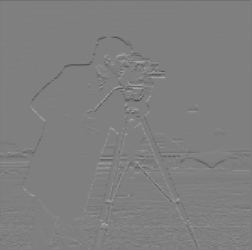
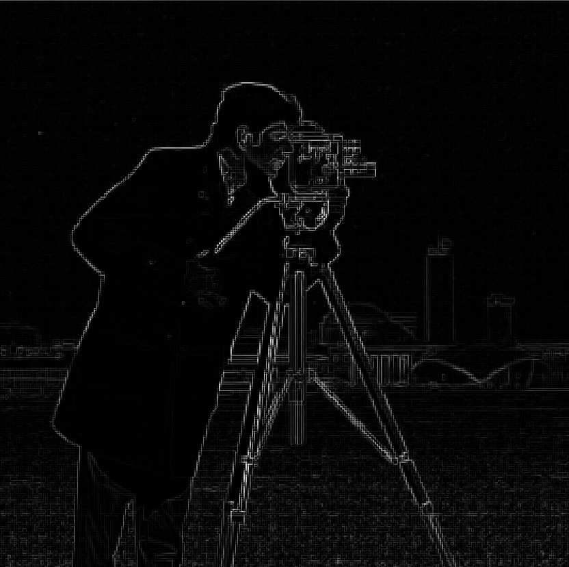
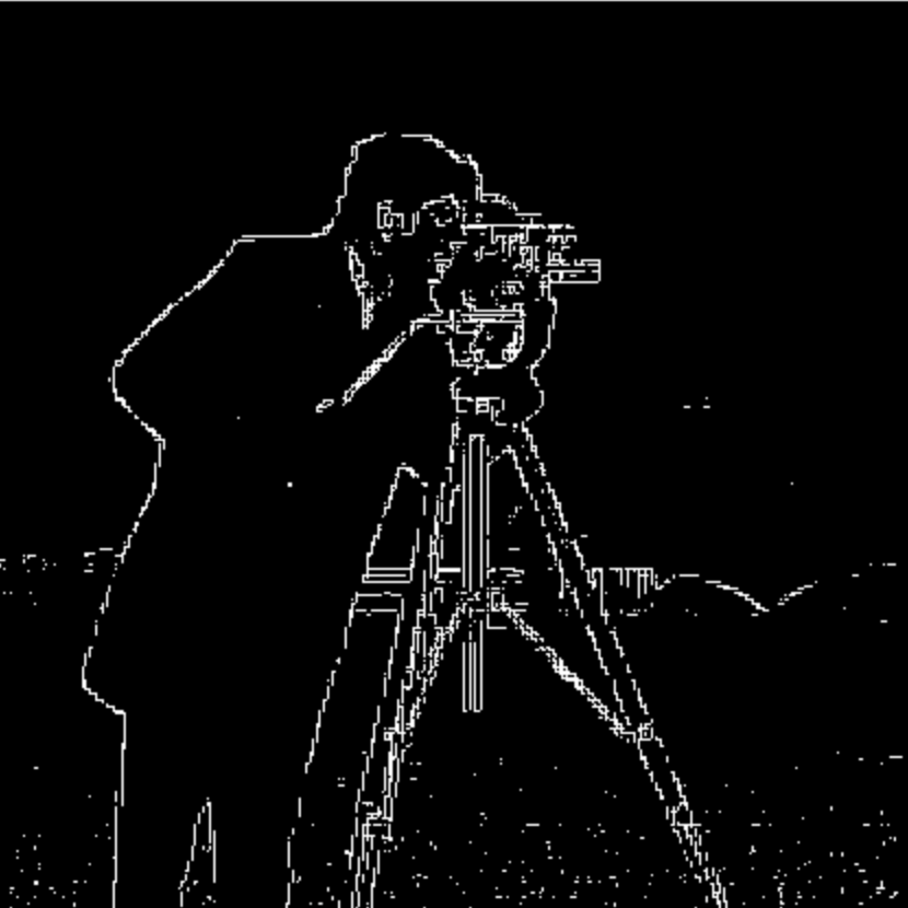
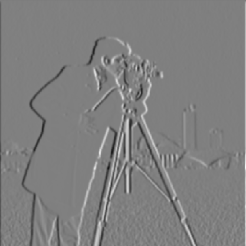
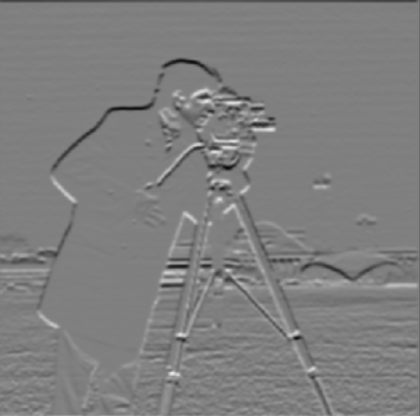
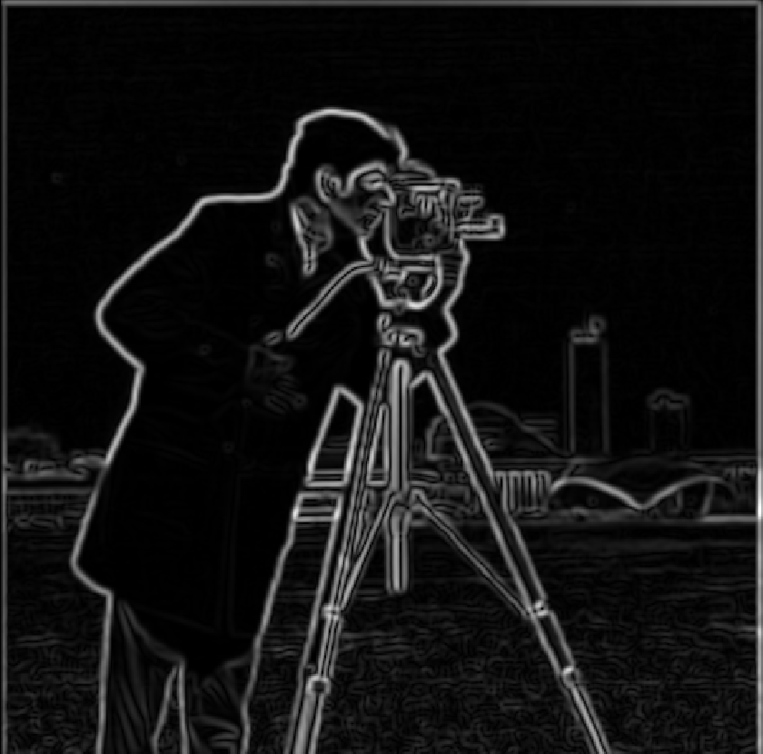
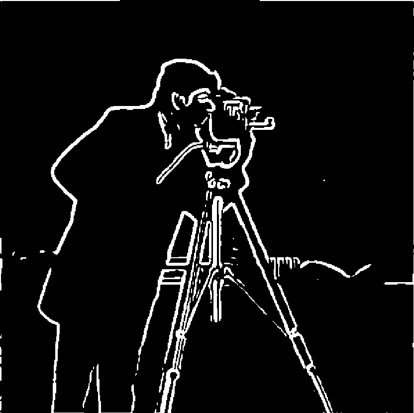
First, I showed the partial derivative in x and y of the cameraman image by convolving the image with finite difference operators D_x = [[1, -1]] and D_y = [[1],[-1]]. To compute the partial derivatives d_x and d_y, I used convolve2d from the scipy.signal library. Then, I computed and showed the gradient magnitude image using this formula: np.sqrt(d_x ** 2 + d_y ** 2). Essentially, I computed the square root of the sum of the squares of the partial derivatives. To turn this into an edge image, I binarized the gradient magnitude image by choosing an appropriate threshold of 0.33 and setting every value above the threshold to be 1 and every value below or equal to the threshold to be 0.


I noticed that the results with just the finite difference operators D_x and D_y were quite noisy so I used a smoothing operator called the Gaussian filter. I created the Gaussian filter by first creating a 1D Gaussian Kernel using cv2.getGaussianKernel(ksize, sigma) with ksize = 10 and sigma = 2. Then, I took the outer product with its transpose to get a 2D gaussian kernel. I then created a blurred version of the original image by convolving it with this gaussian kernel. Once I have the blurred image, I repeat the procedure in the previous part with threshold = 0.055 to create the gradient magnitude image and the binarized gradient magnitude image.
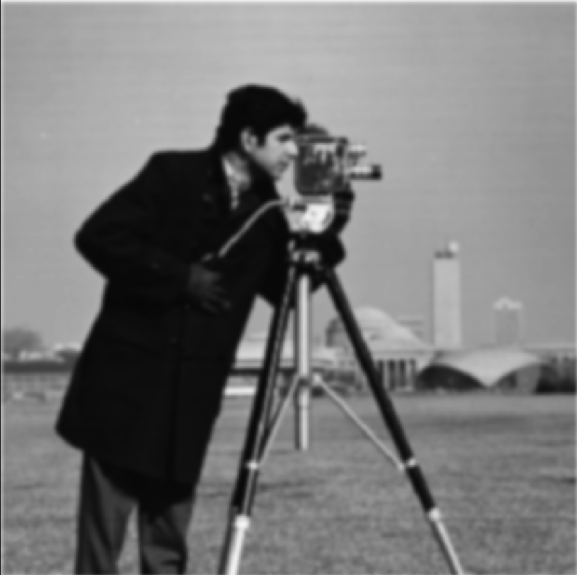
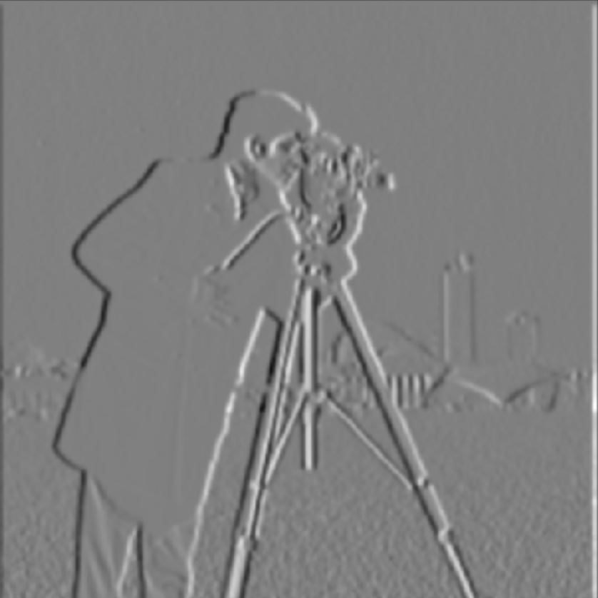
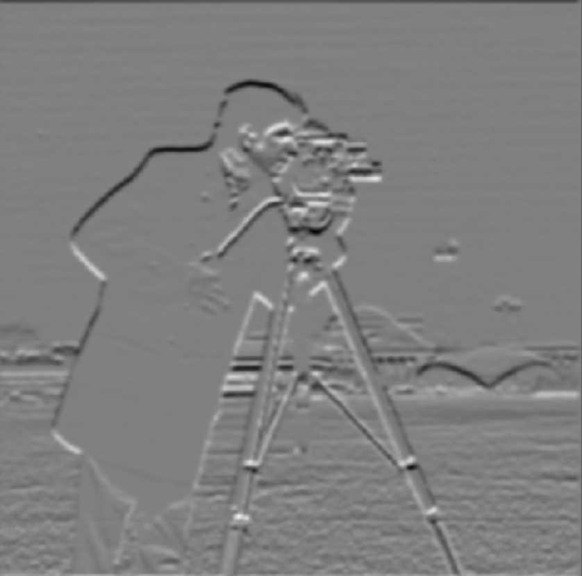
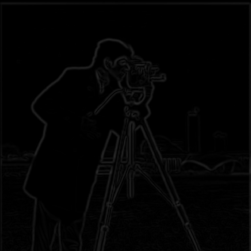
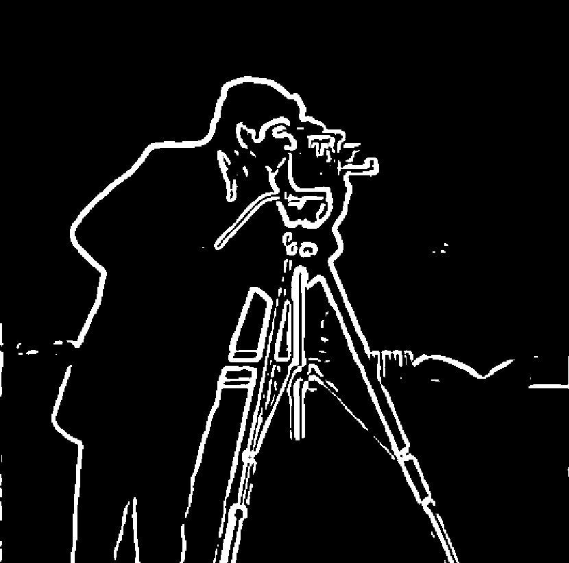
I see the following differences:
To help me build intuition that convolutions are associative, I now do the same thing with a single convolution instead of two by creating a derivative of Gaussian filters. First, I convolve the Gaussian with D_x and D_y. Then, I display the resulting DoG filters as images. As can be seen, I verify that I get the same results as in the previous step, therefore proving that convolutions are associative.

In this part, we will derive the unsharp masking technique. The Gaussian filter is a low pass filter that retains only the low frequencies. Therefore, if we subtract the blurred version from the original image, we can get the high frequencies of the image. We combine this all into a single convolution operation which is called the unsharp mask filter. To construct this filter, I first created a 2D Gaussian kernel using kernel size 10 and sigma value 2 and convolved it with the original image to produce a blurry image that contains the low frequencies of the image. Then, I subtract the blurry image from the original image to produce an image that contains the high frequencies of the image. To create the sharpened image, I uses the following formula: original image + (alpha * high frequency image) where increasing alpha increases the number of high frequency images added to the original image, which makes the image sharper.

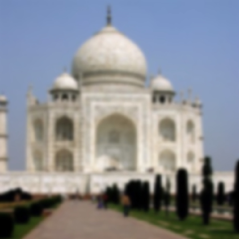
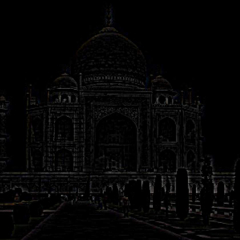
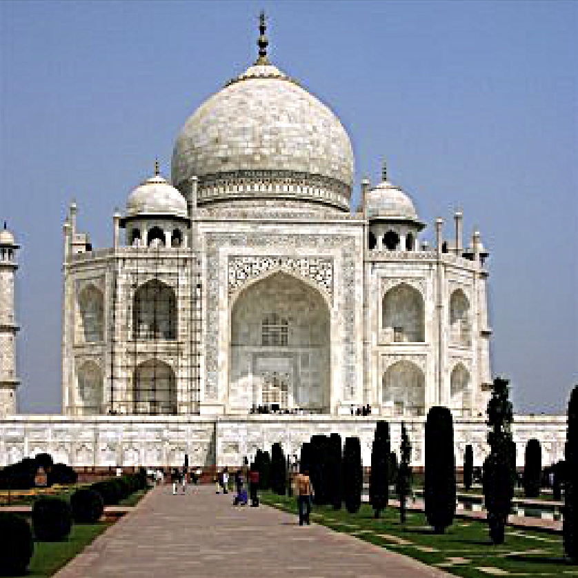
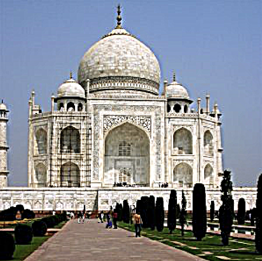
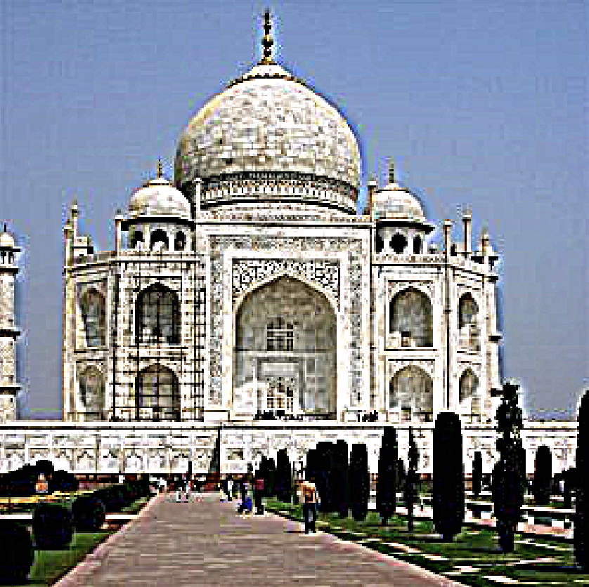
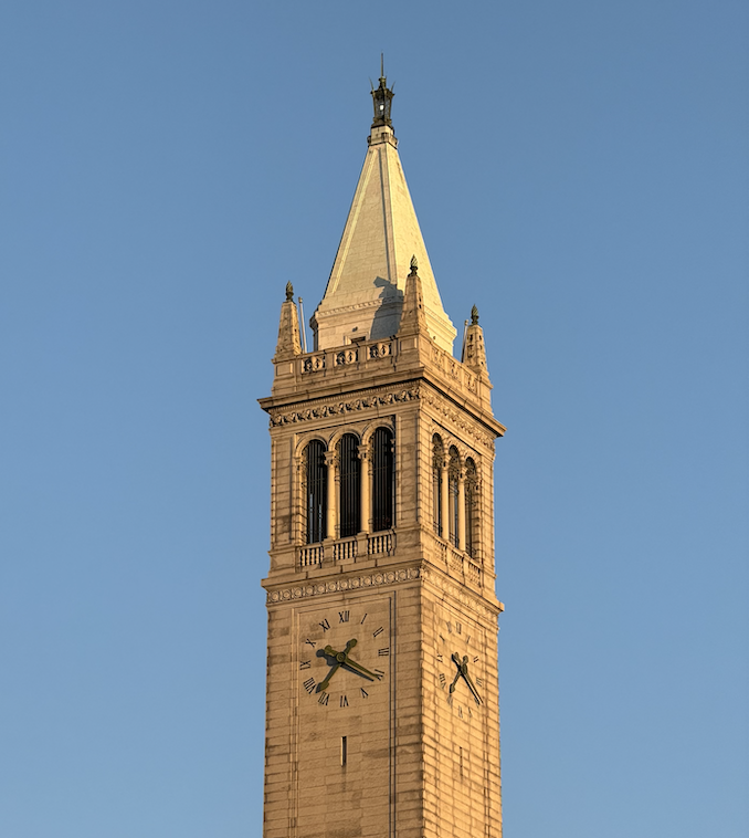
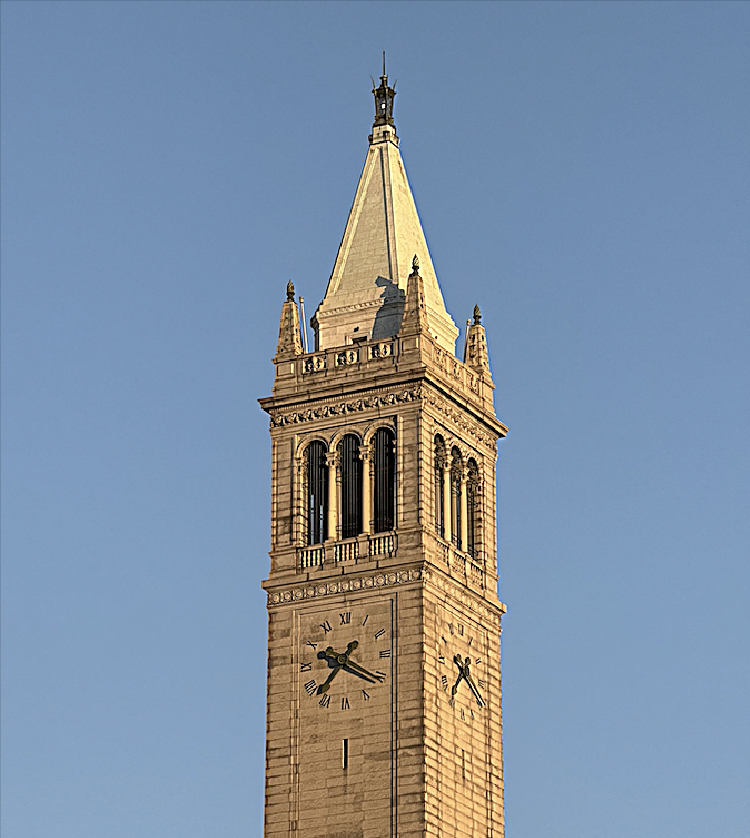
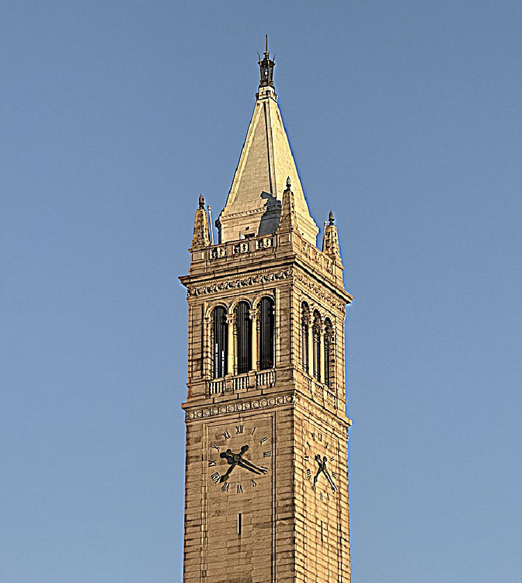
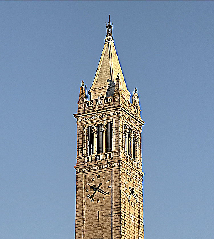
Here is a sharp image that I blurred and then sharpened again:
The goal of this part of the assignment is to create hybrid images using the approach described in the SIGGRAPH 2006 paper by Oliva, Torralba, and Schyns. Hybrid images are static images that change in interpretation as a function of the viewing distance. The basic idea is that high frequency tends to dominate perception when it is available, but, at a distance, only the low frequency (smooth) part of the signal can be seen. By blending the high frequency portion of one image with the low-frequency portion of another, you get a hybrid image that leads to different interpretations at different distances.
Here are the sample images I used for debugging and the hybrid image produced from them:
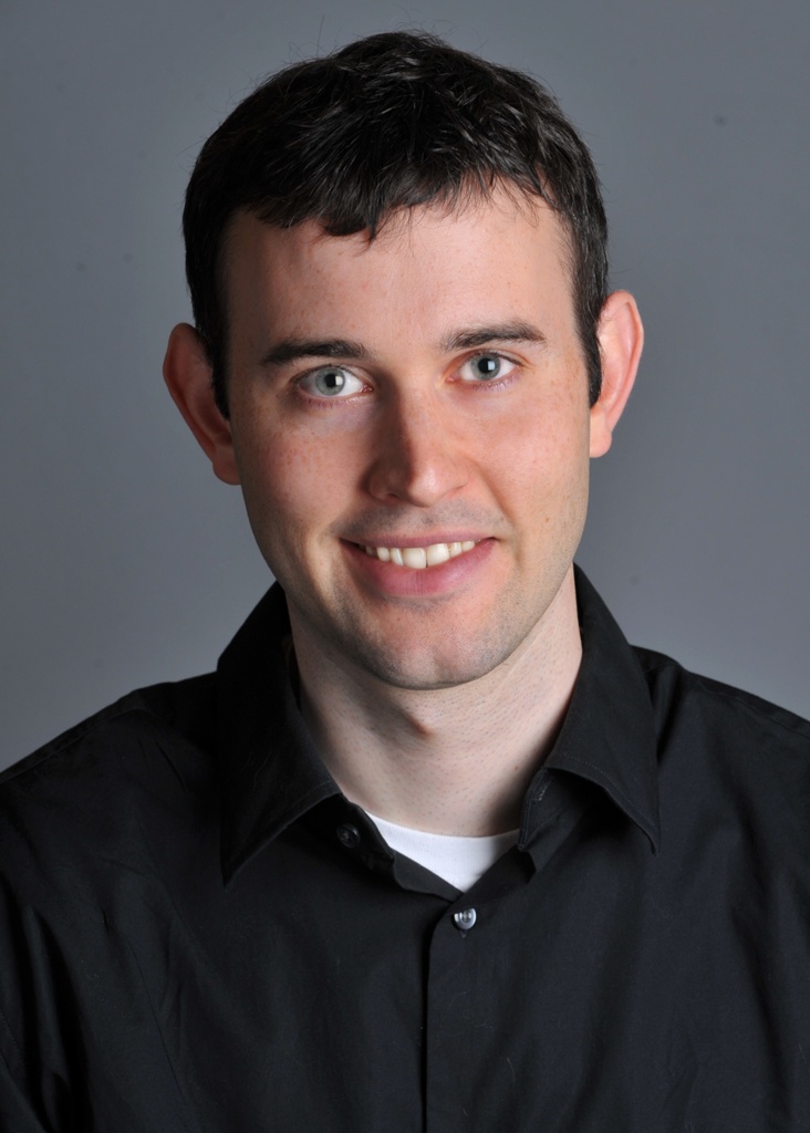
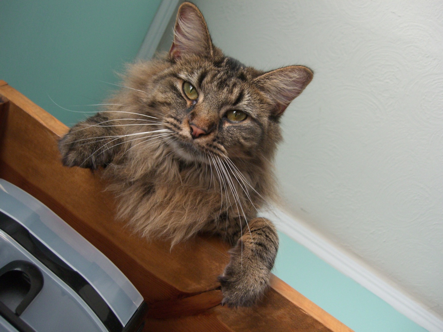
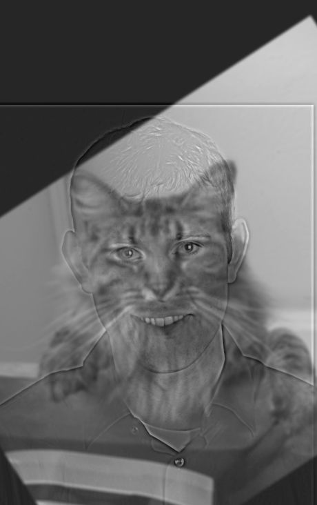
In order to create this hybrid image, I wrote code to low-pass filter one image by using a Gaussian filter, high-pass filter the second image by subtracting the blurred image from the original image, and then averaged the two images to produce the final hybrid image. For a low-pass filter, Oliva et al. suggested using a standard 2D Gaussian filter. For a high-pass filter, they suggest using the impulse filter minus the Gaussian filter (which can be computed by subtracting the Gaussian-filtered image from the original). I chose the cutoff-frequency of each filter by doing some experimentation.
Here, I combine Nadal and Federer into a hybrid image. At closer distances, you see Nadal but at further distances you see Federer.
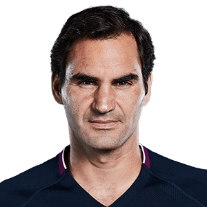
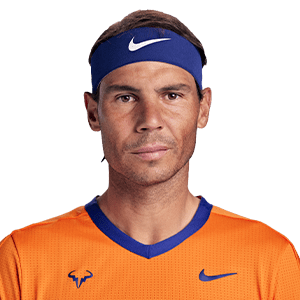
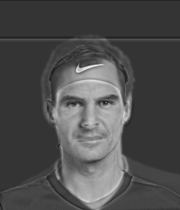
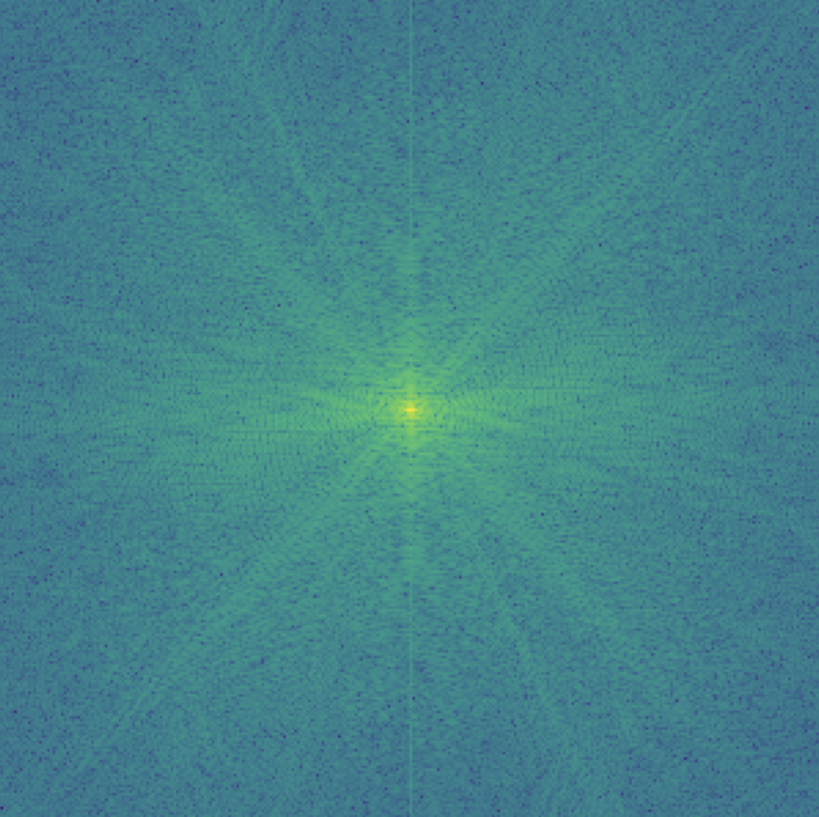
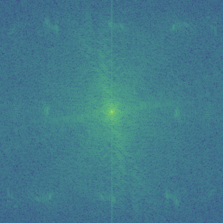
My favorite result is this hybrid image of Nadal and Federer so I also illustrated the process through frequency analysis. I showed the log magnitude of the Fourier transform of the two input images, the filtered images, and the hybrid image using: plt.imshow(np.log(np.abs(np.fft.fftshift(np.fft.fft2(gray_image)))))
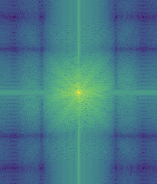
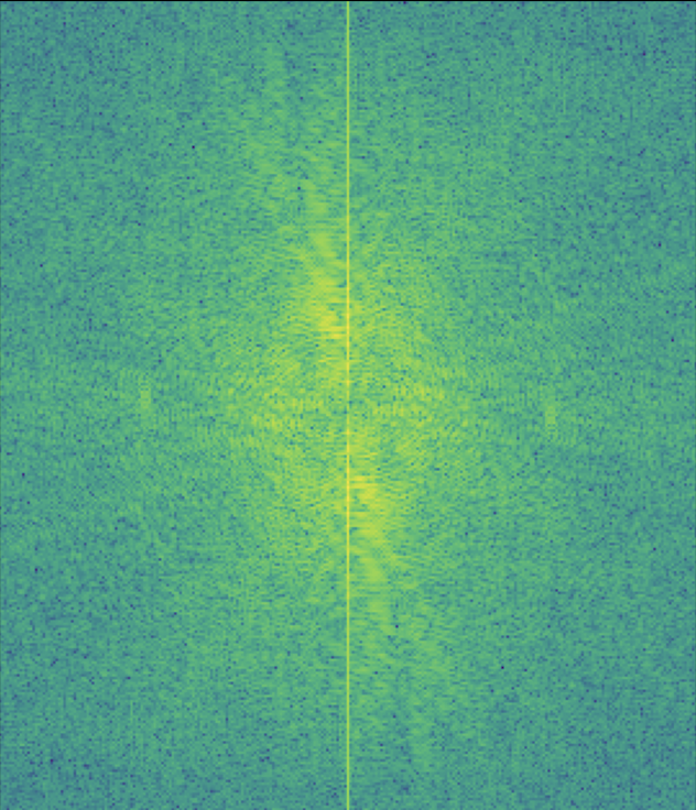
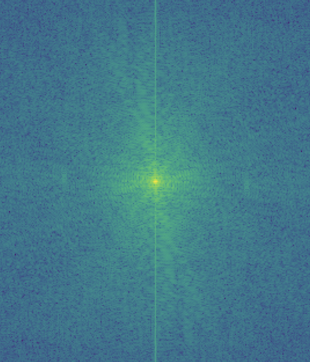
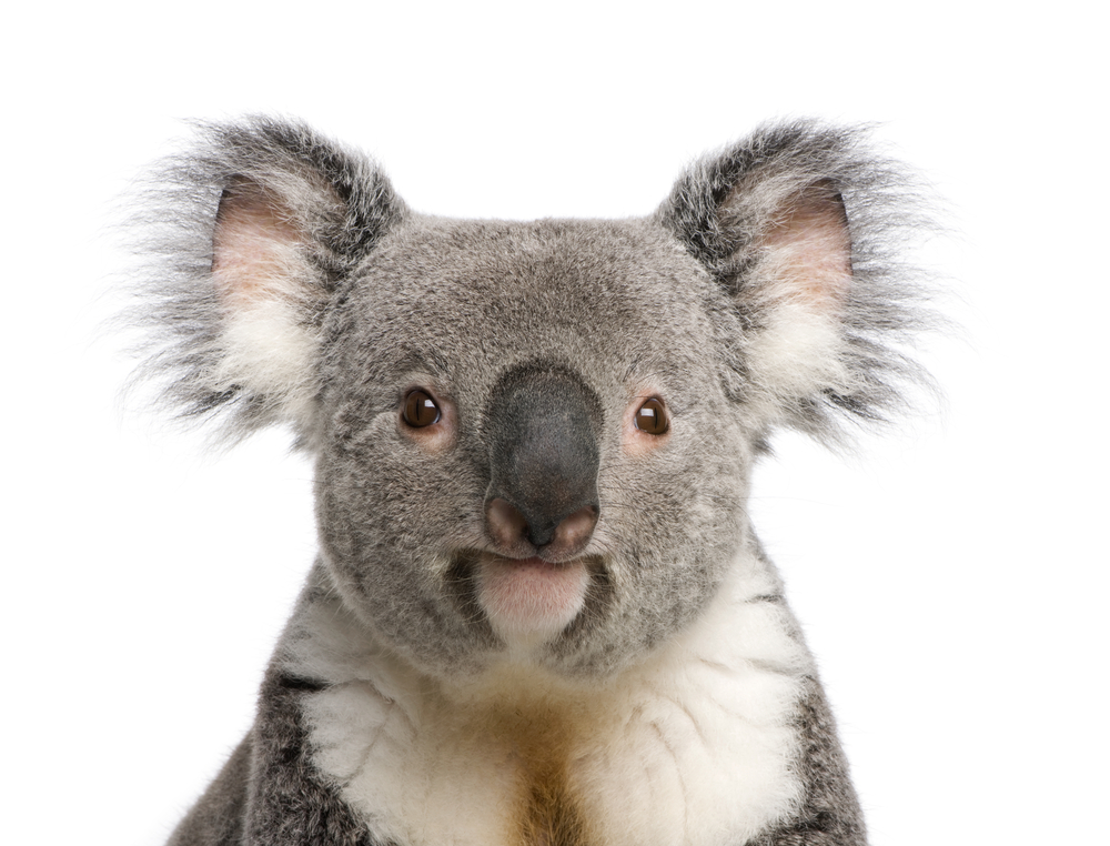
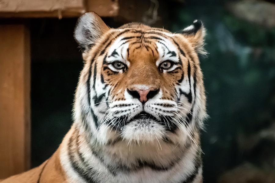
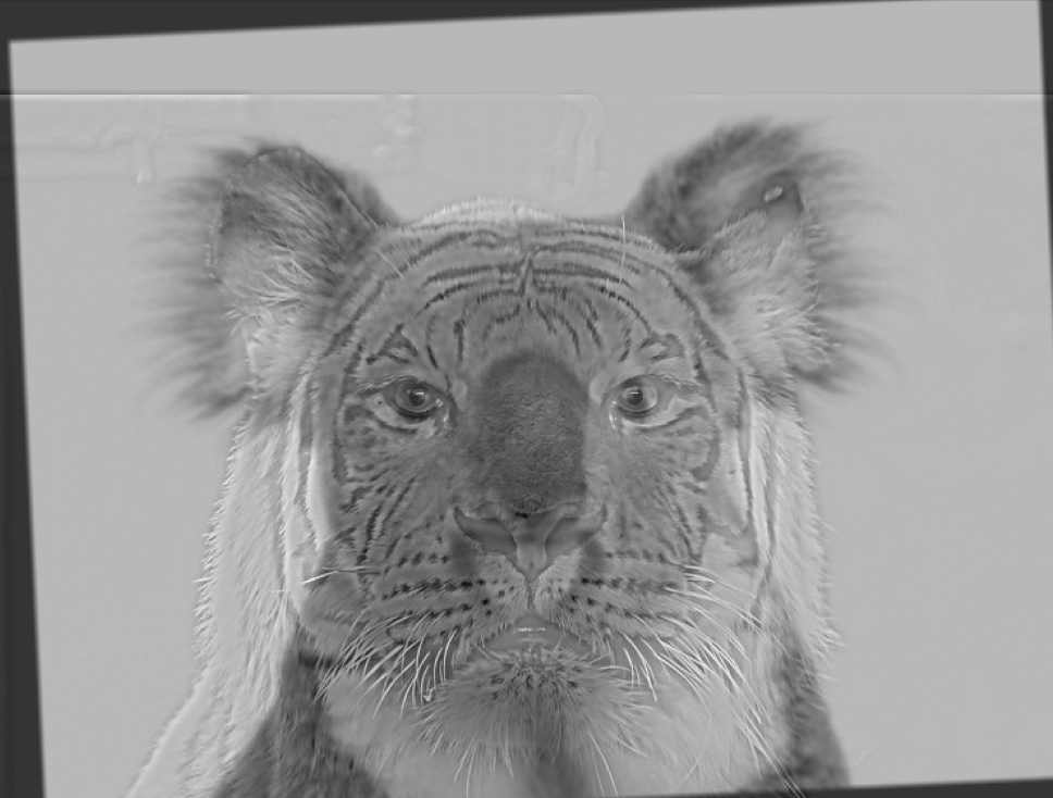
Here is an example of a failure case. I tried to combine a koala and a tiger but it is quite difficult to see the tiger at close distances since the koala dominates the image. Maybe I could try using color to enhance the effect and instead of choosing a tiger, maybe I should've chosen something that is more similar in shape to a koala.
The goal of this part of the assignment is to blend two images seamlessly using multi resolution blending as described in the 1983 paper by Burt and Adelson. An image spline is a smooth seam joining two image together by gently distorting them. Multiresolution blending computes a gentle seam between the two images seperately at each band of image frequencies, resulting in a much smoother seam. First, I need to create and visualize the Gaussian and Laplacian stacks and then using the stacks, I need to blend together images. Firstly, for this part I need to implement the Gaussian and Laplacian stacks, which are similar to pyramids but without the downsampling. In order to build the Gaussian stack, I use a for loop to iterate through each level and produce an image that is blurrier than the previous level using a 2D Gaussian filter. As a result, the higher the level, the more blurry the image is. In order to build the Laplacian stack, I use a for loop to iterate (levels - 1) times, each time producing an image that is equaivalent to subtracting the blurrier image at the next level from the image at the current level. The last level of the Laplacian stack is the same as the last level of the Gaussian stack. Constructing the Gaussian and Laplacian stacks will prepare me for the next step of Multi-resolution blending in the next section.


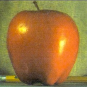
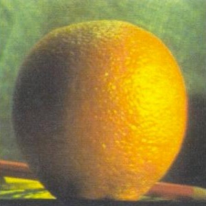
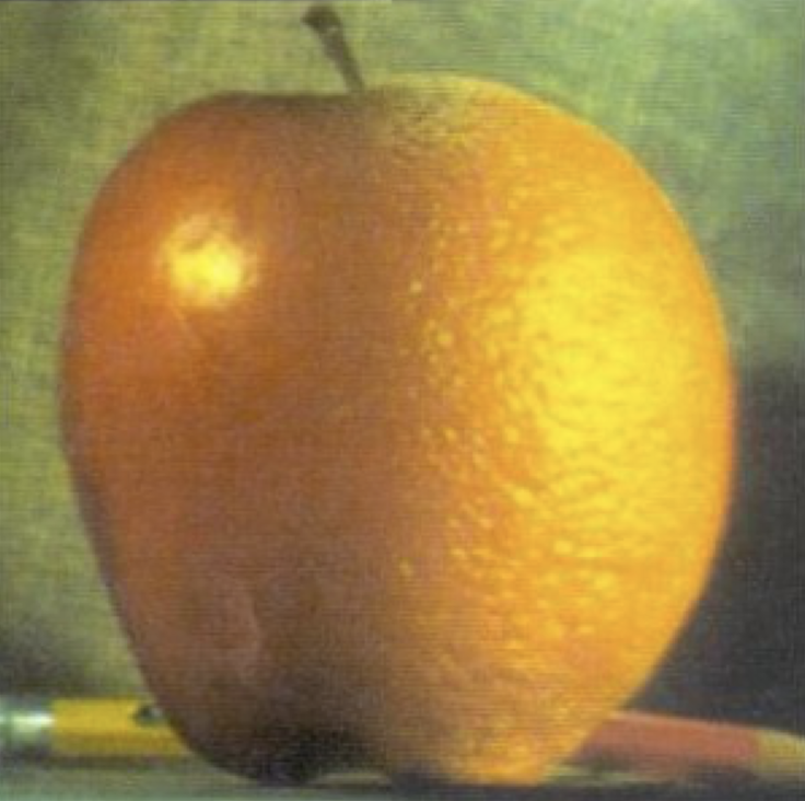
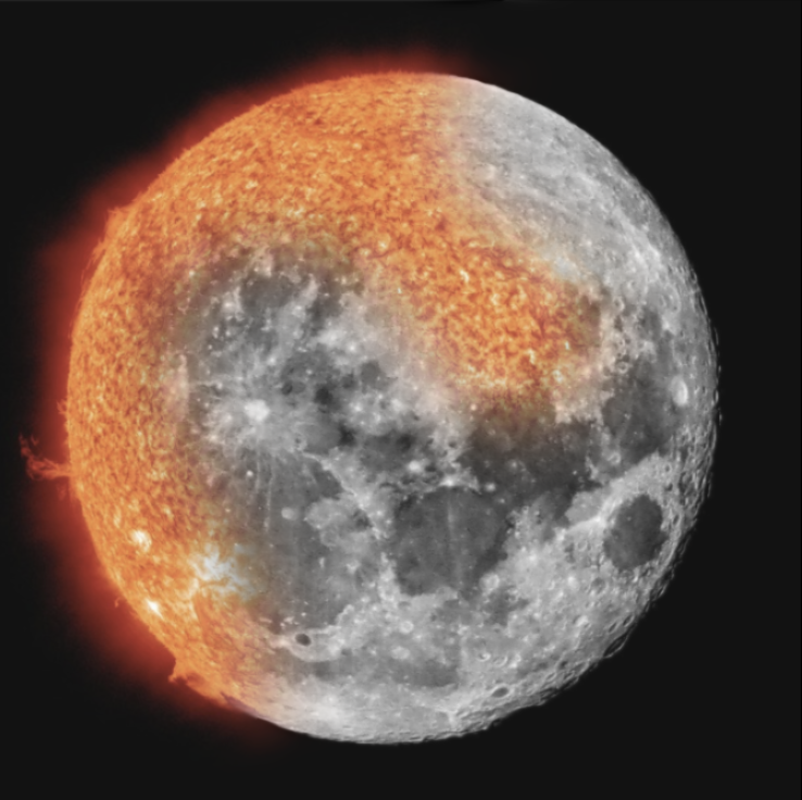
In this part, we will mainly focus on blending two images together. After constructing the Gaussian and Laplacian stacks for the two images, we need to construct the Gaussian stack for the mask which will help blur the seam between the two images. Then, in order to create the blended image, I use this formula: blended = (1 - gaussian_stack_mask) * laplacian_stack_apple + gaussian_stack_mask * laplacian_stack_orange. This creates a Laplacian stack for the hybrid image so then we need to add all the layers together to get the final blended image.
Here are the sample images I used for debugging:
