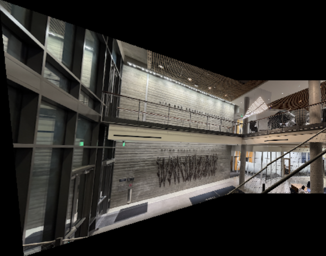
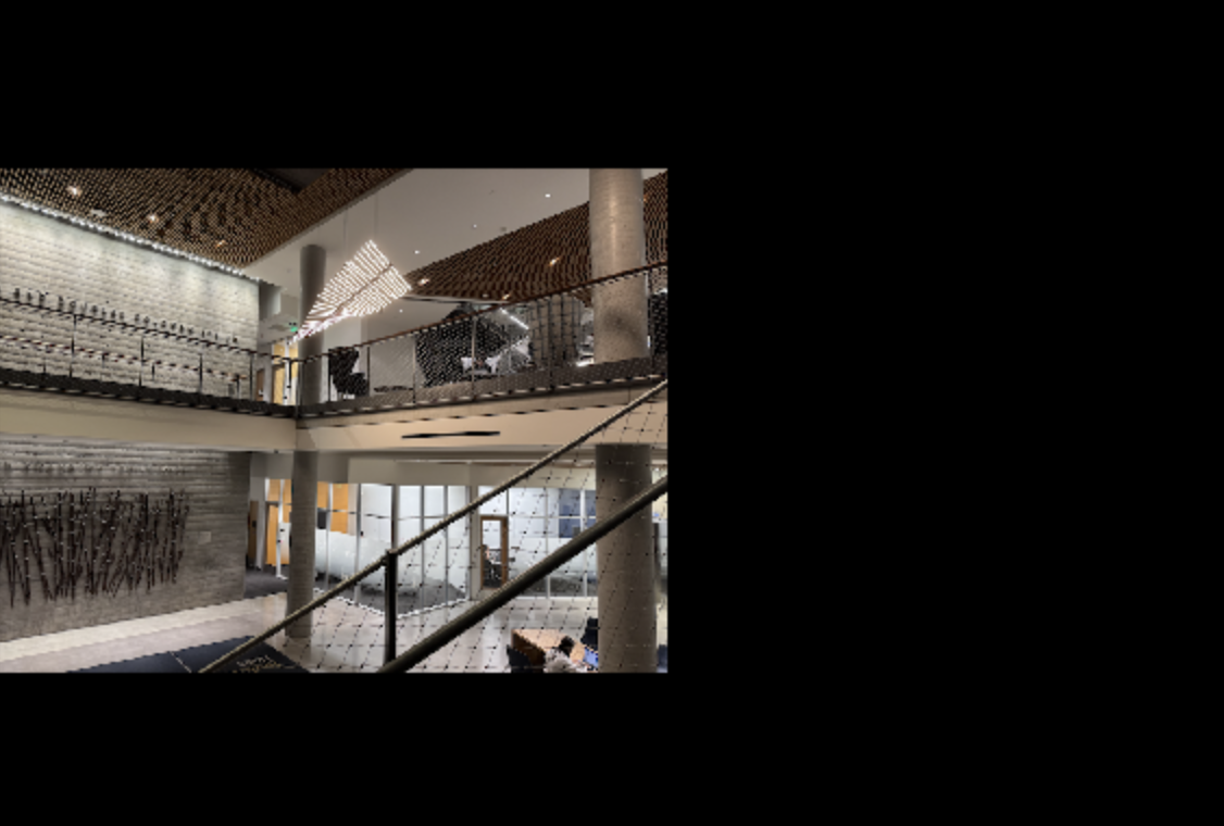
Hildebrand Left
Hildebrand Center
Hildebrand Right
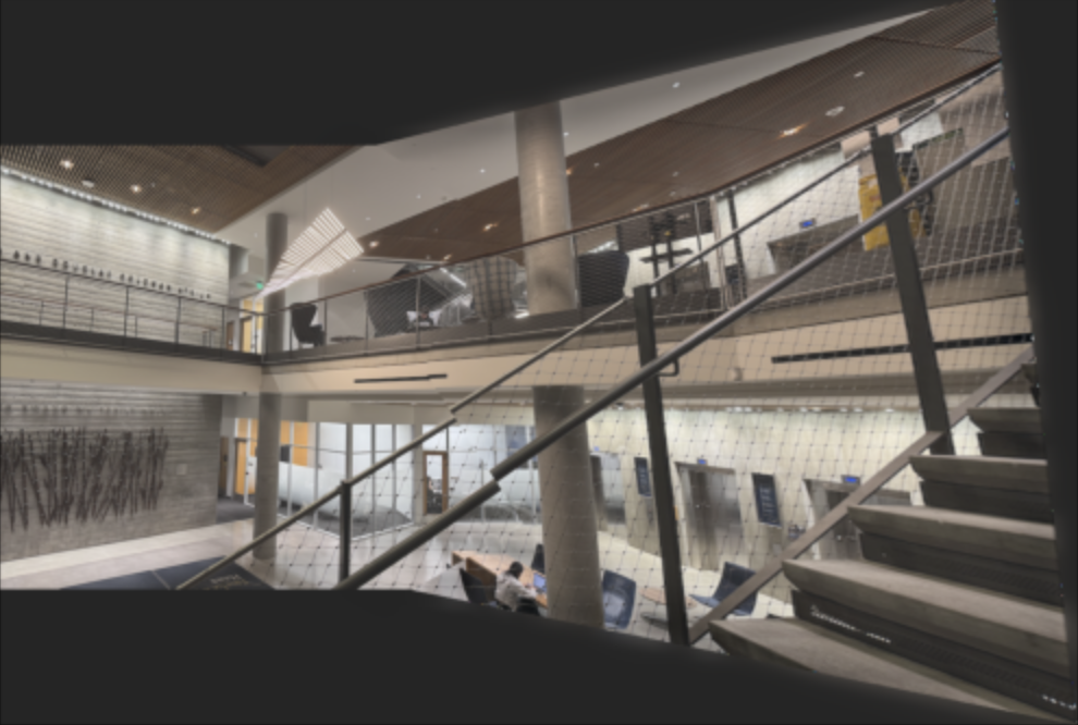
In this project, I take two or three photographs and create an image mosaic by registering, projective warping, resampling, and compositing them. Throughout this project, I learned how to compute homographies, and use them to warp images.
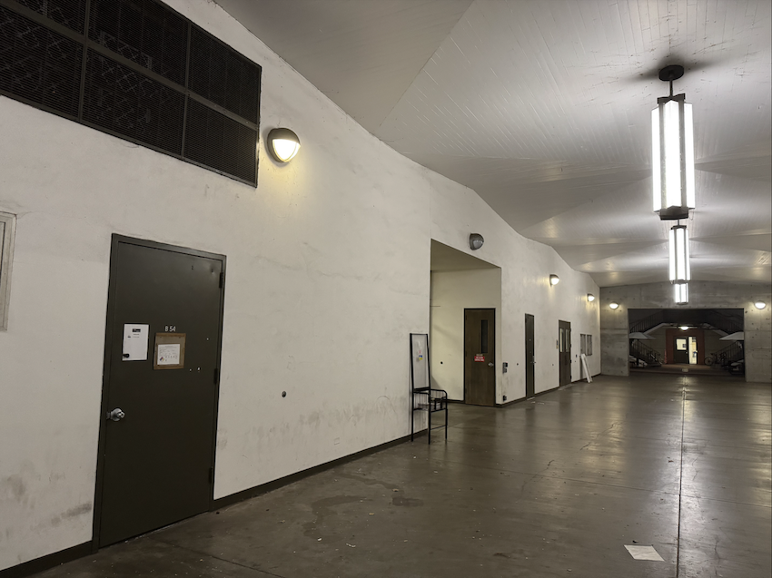
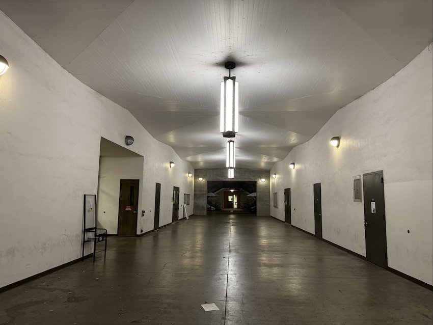
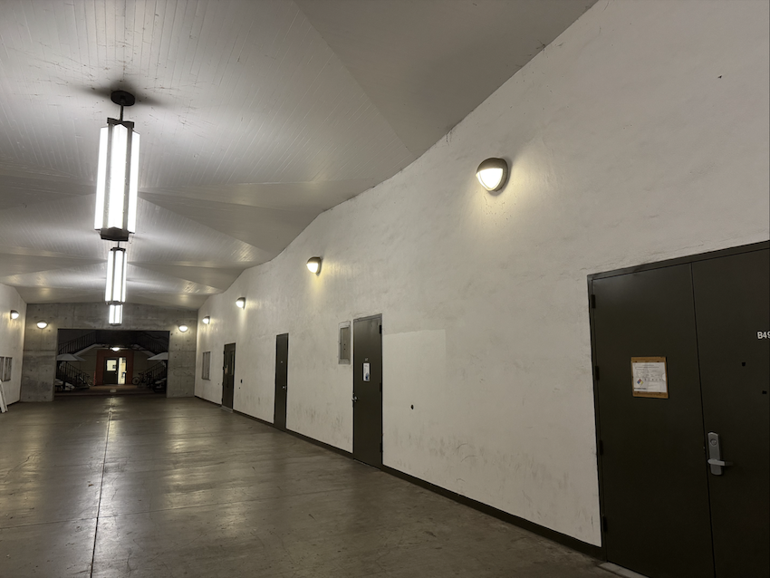
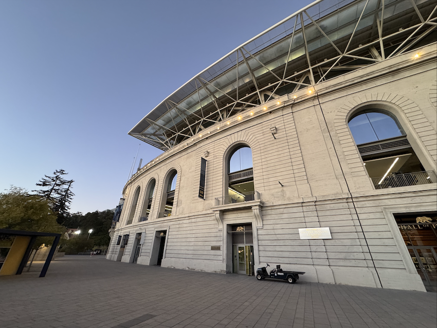
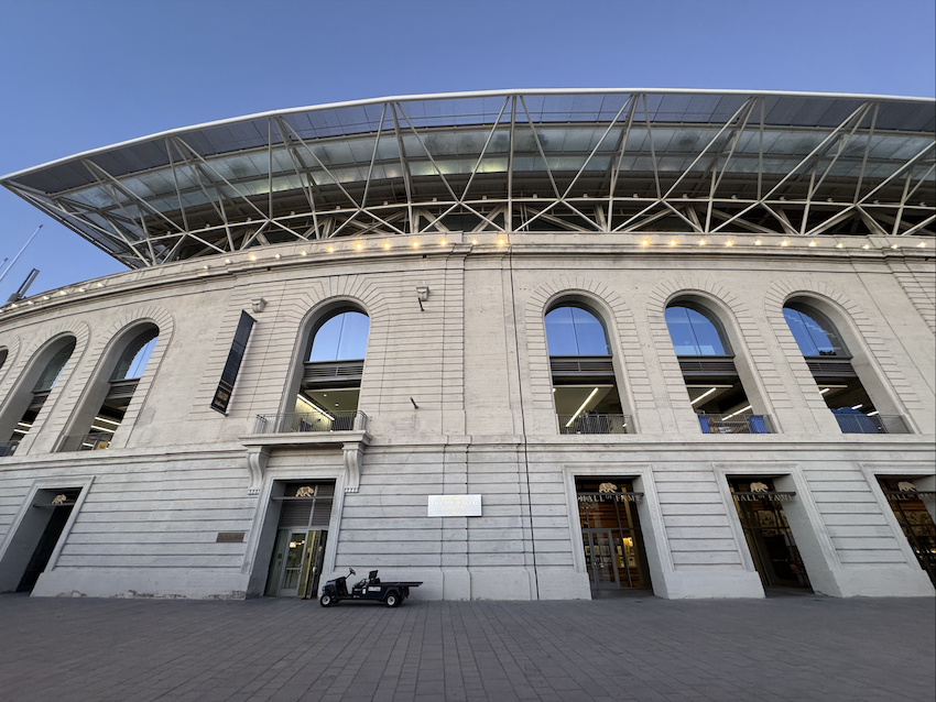
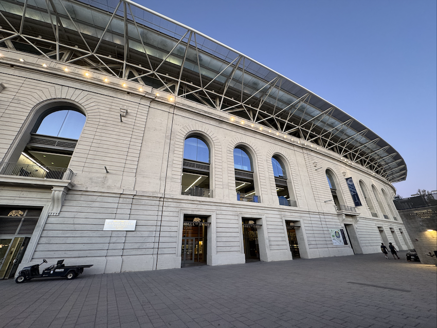
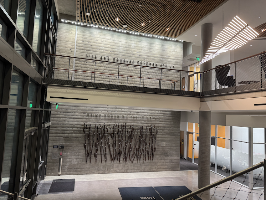
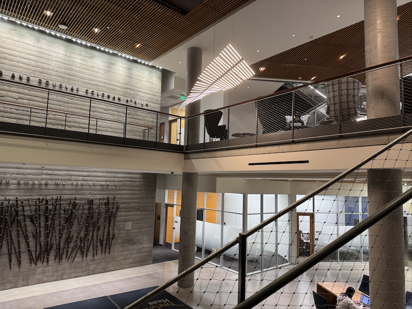
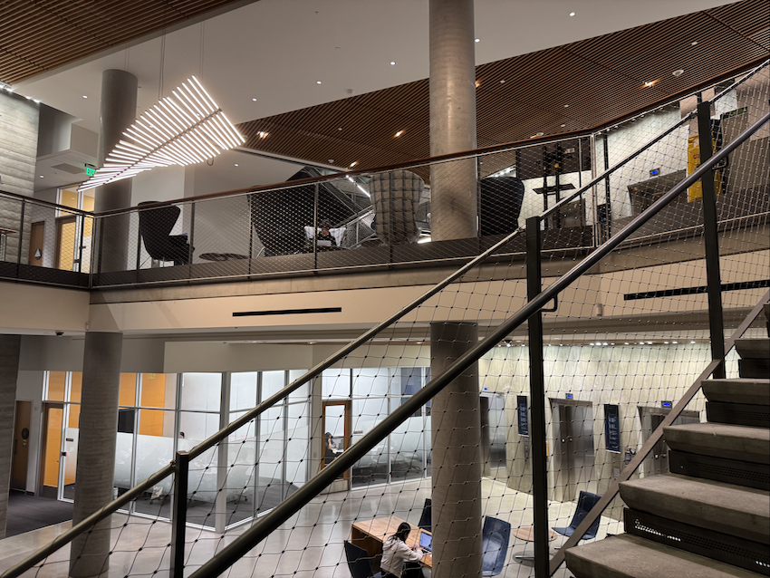
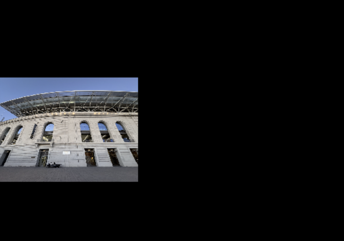
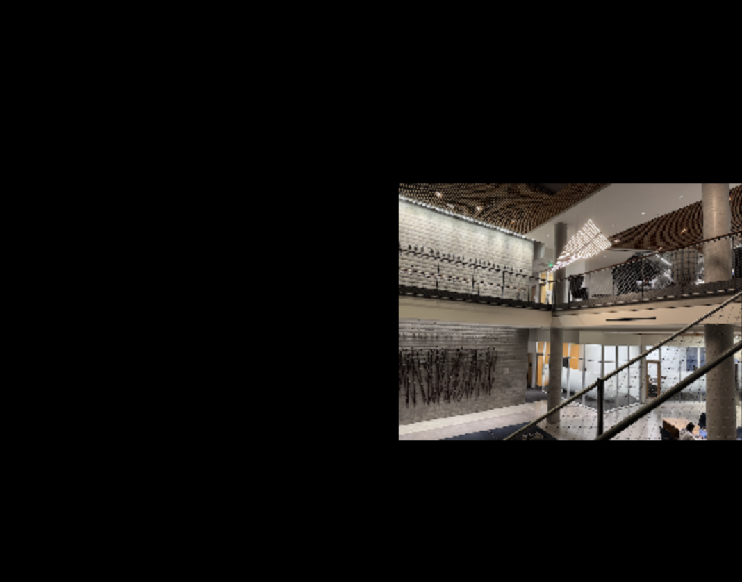
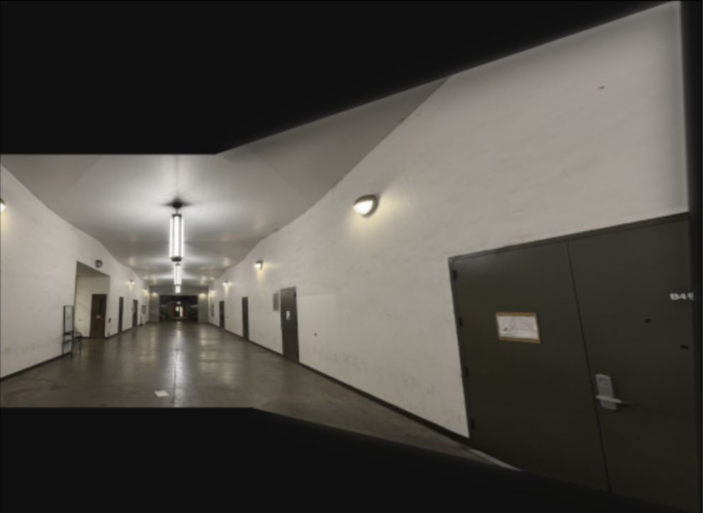
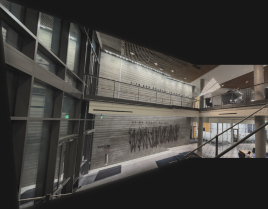
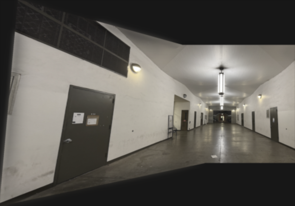
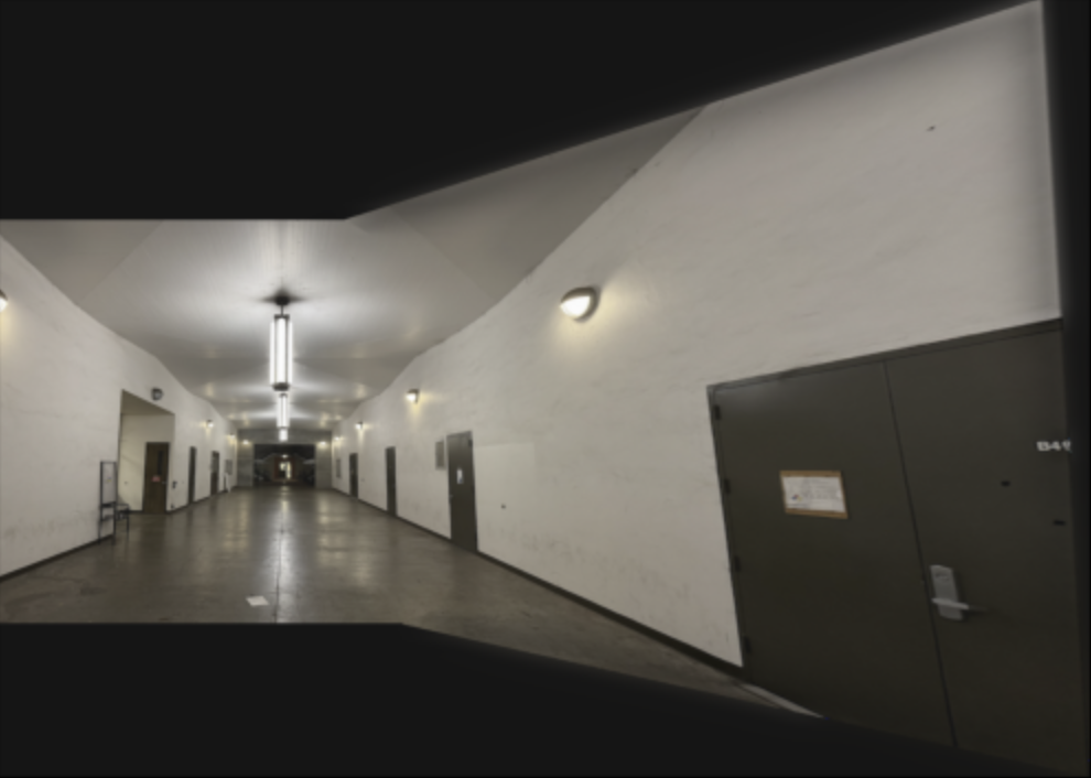
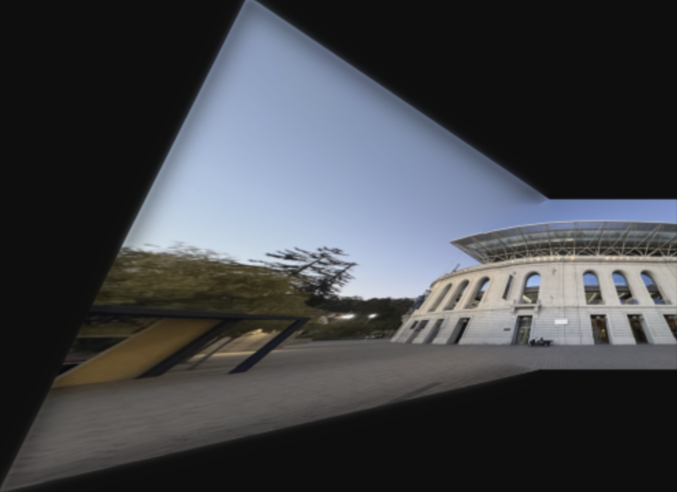
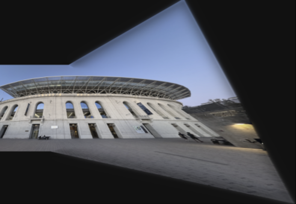
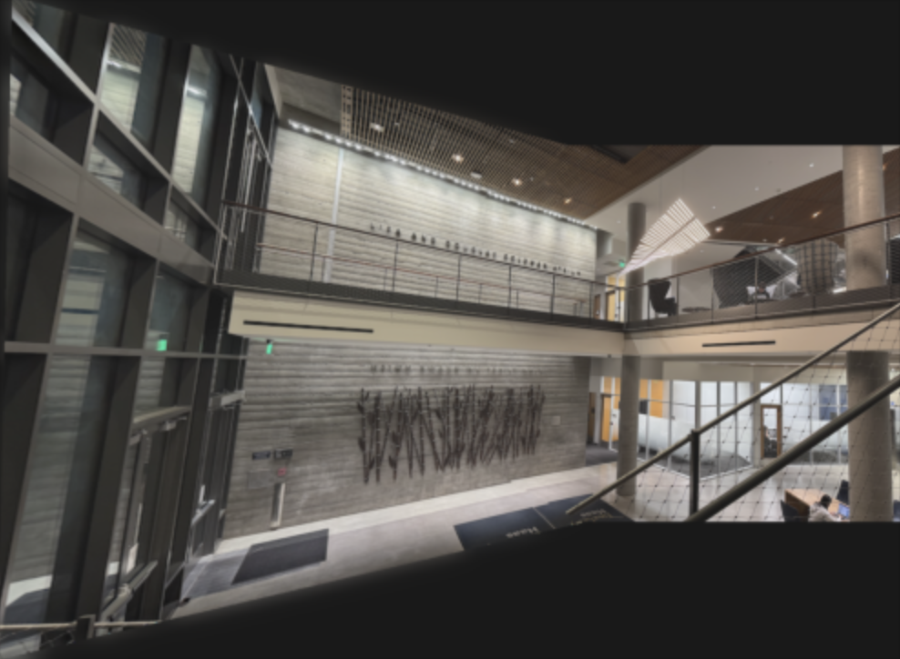
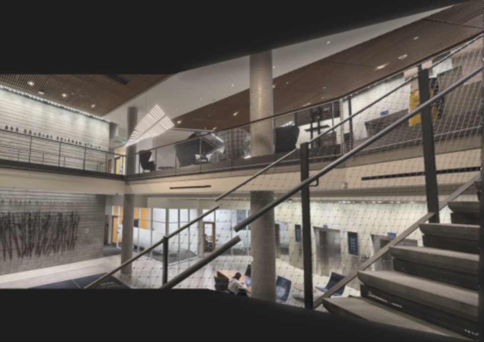
Below are some images I used in this project:
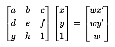
First, using the online tool provided by the course, I identified correspondence points in each pair of images, where one image is the image that will be warped onto the reference image and the second image is the reference image. We want to find a 3x3 matrix, H, to compute a projective transformation, as shown on the left image. On the right image, we see how we can rearrange the equations to solve for our H matrix:
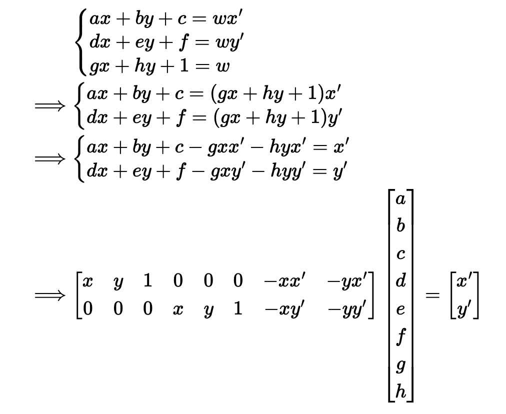
After setting up the overdetermined linear system of equations, we solve it using least squares. After performing SVD, we get the matrices U, S and V transpose. In order to minimize the loss function, we want the vector that corresponds to the smallest eigenvalue in V transpose, which is the last vector, since the vectors are ordered in decreasing magnitude. Once we have solved for all the unknown values of the H matrix, we reshape the 9x1 vector into a 3x3 matrix. This becomes our H matrix.
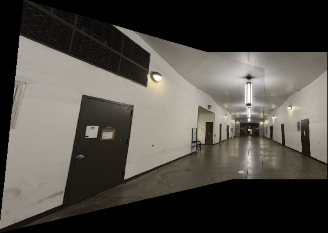
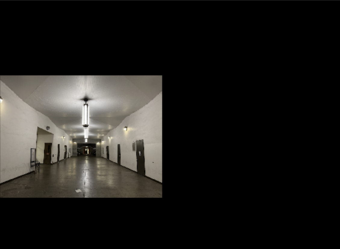
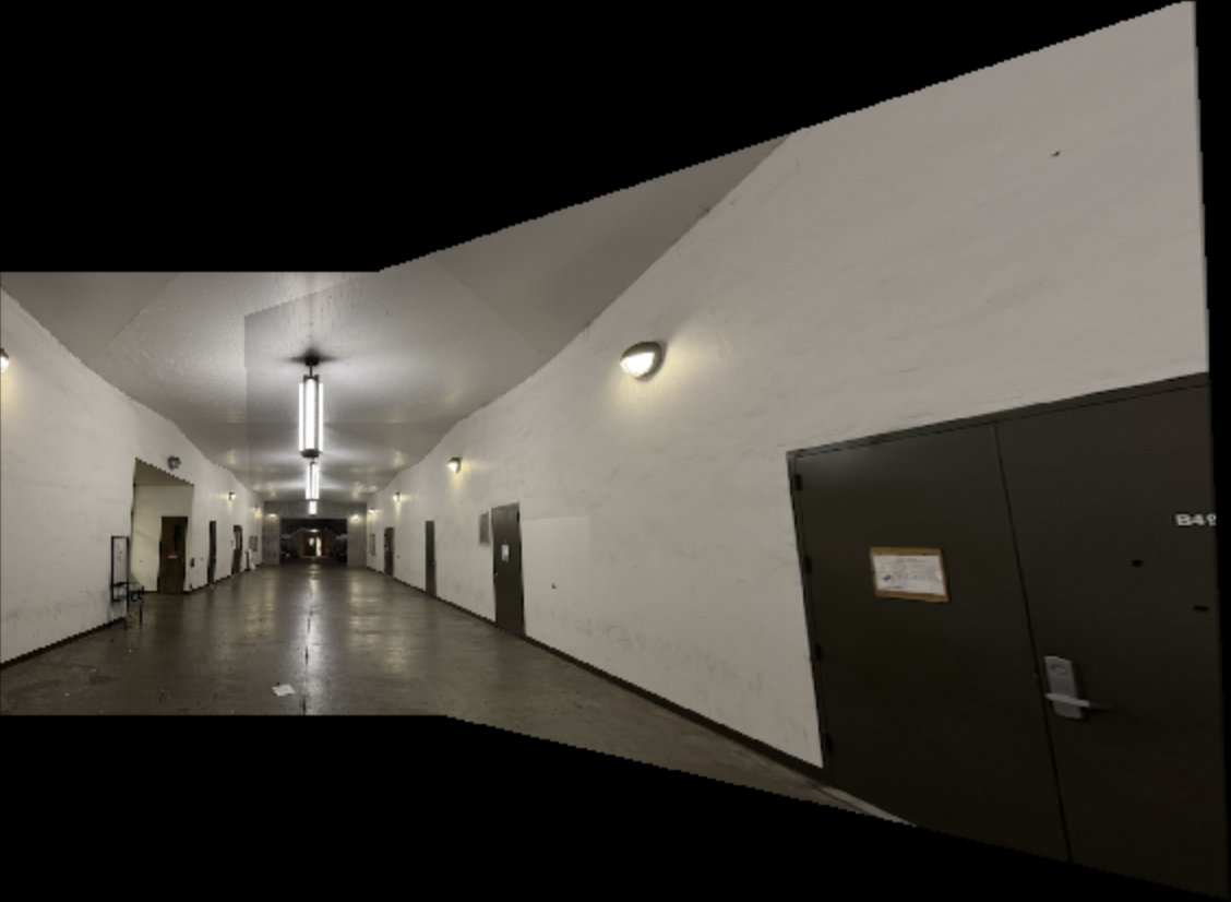
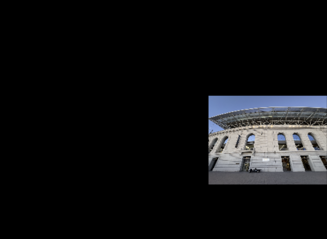
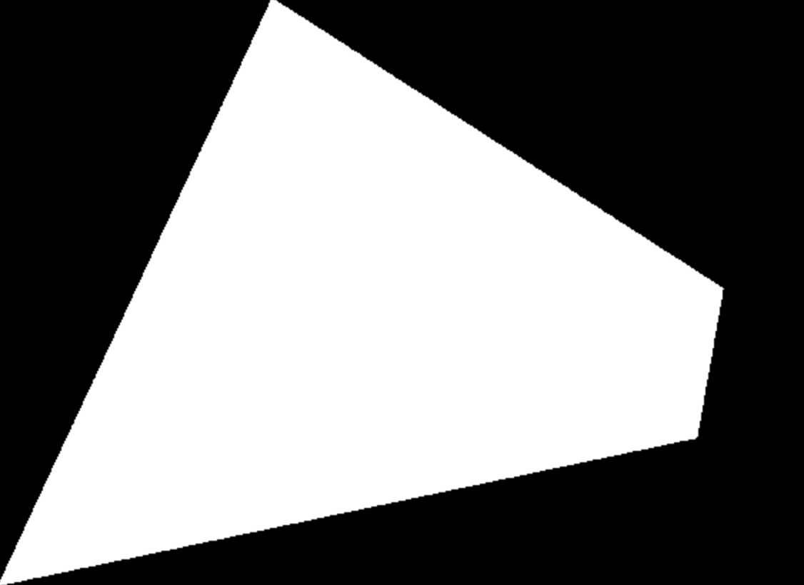
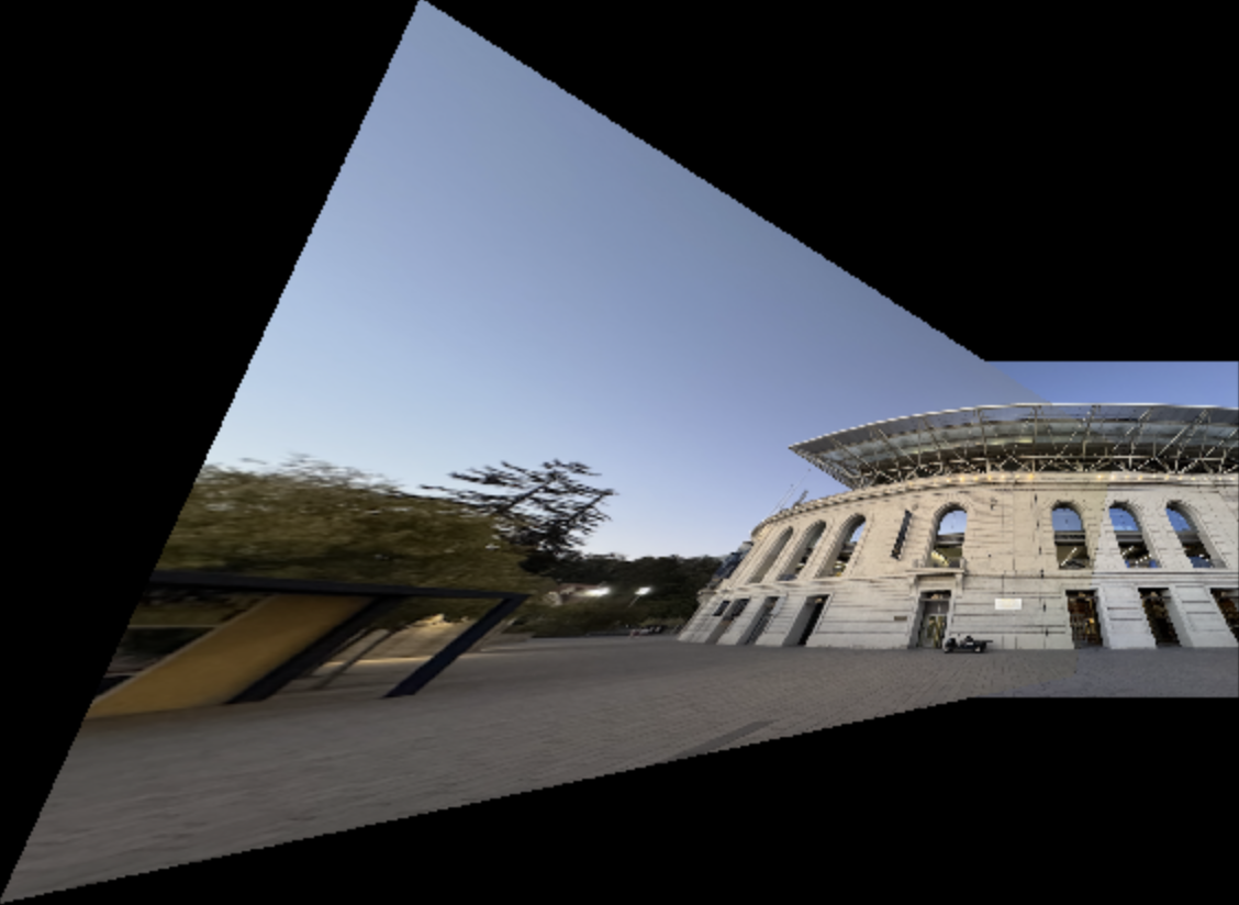
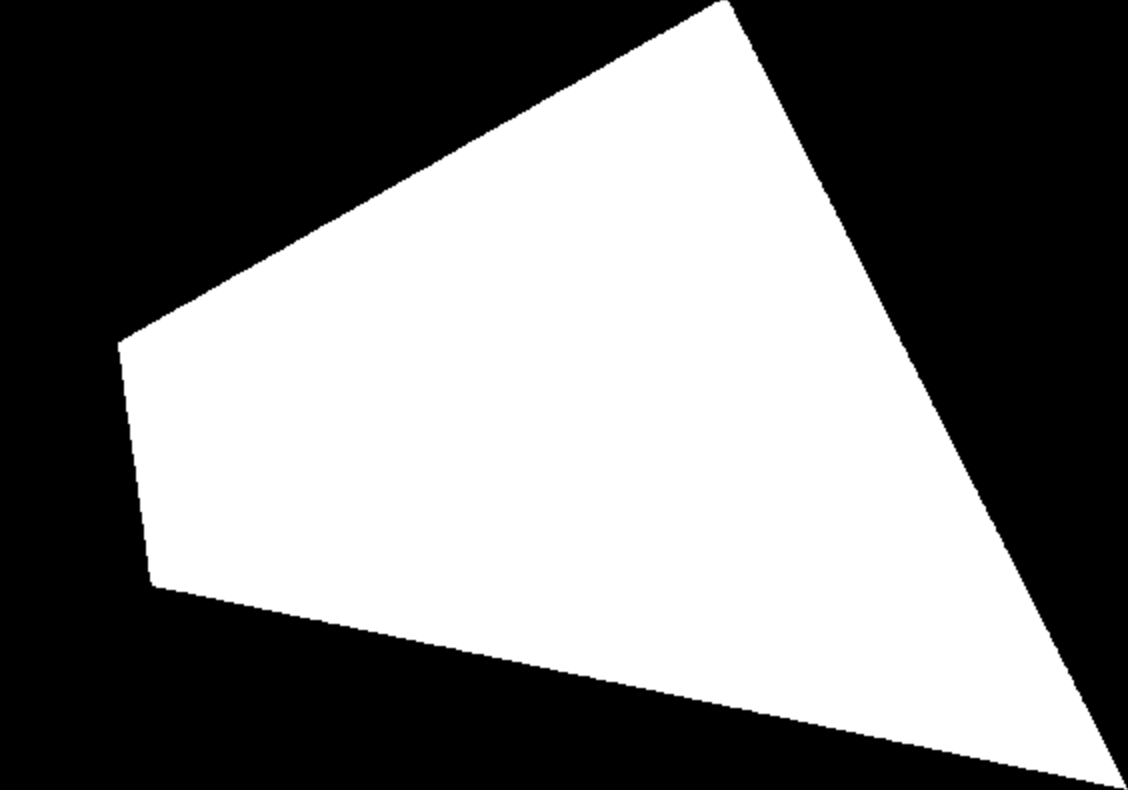
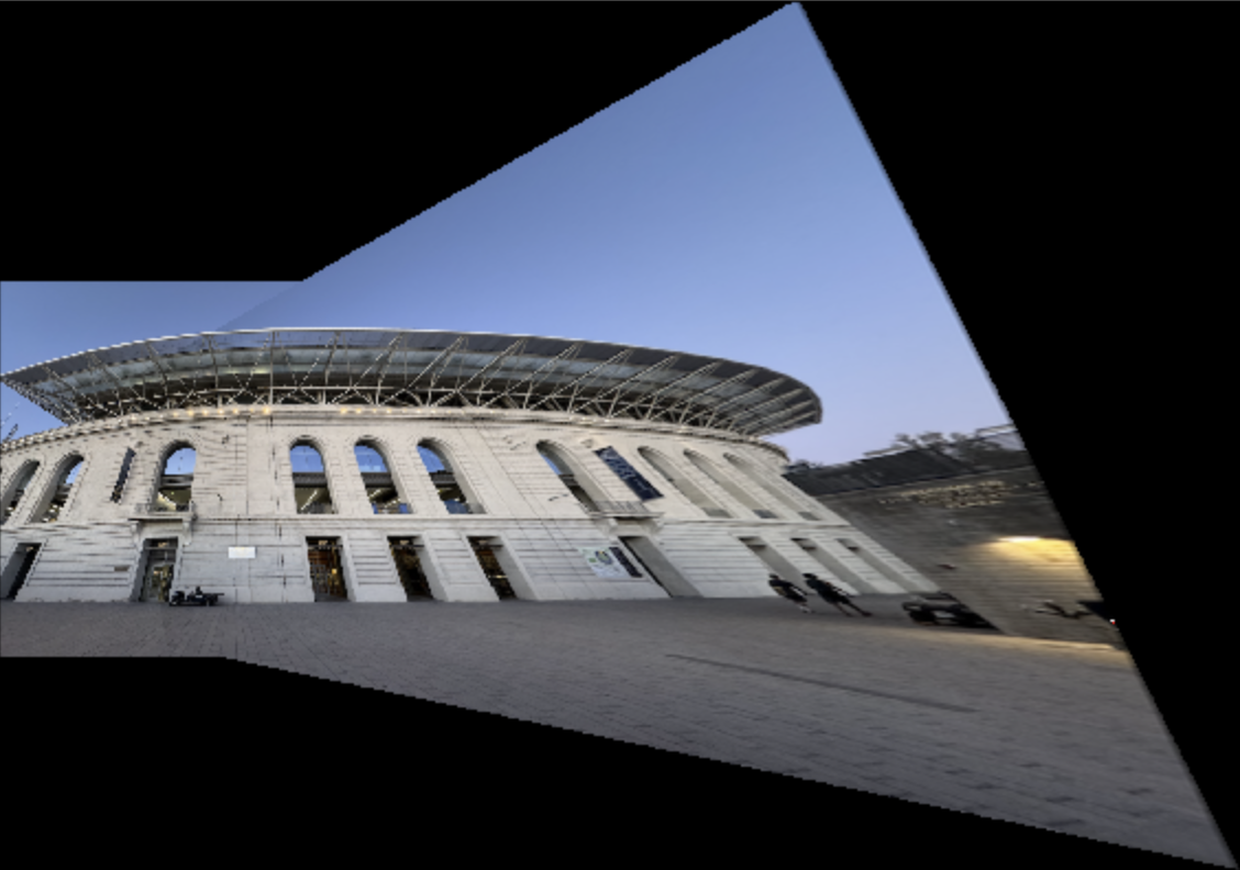
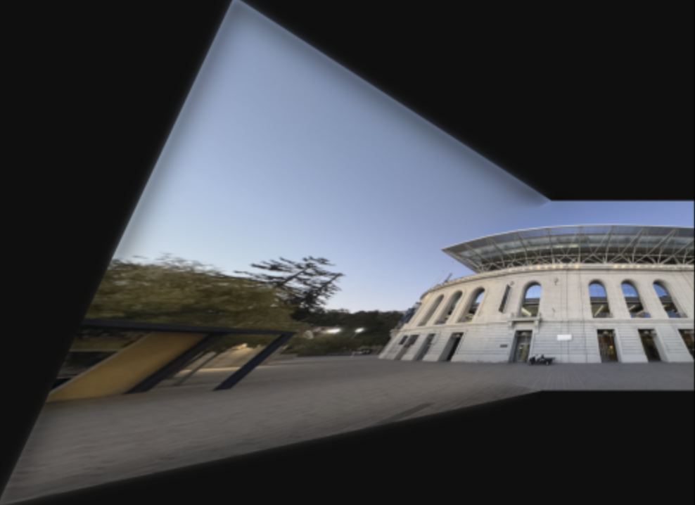
Now that we have calculated the homography matrix, we can use it to warp each image towards the reference image. First, I find the corners of the first image to identify the boundaries of the bounding box before warping. Then, I do a forward warp of the bounding box and normalize it so that I know the space in which the pixels need to be filled. I then find the bounding box of the final image, which is an empty canvas so I copy over image 2 into the final output. Once I've found the polygon in which the final image will be placed, I applied inverse homography to perform a backward warp to produce the final output coordinates of the warped image 1. Finally, I interpolated the pixels in image 1 that will be mapped to each pixel in the output. Below are the resulting images:
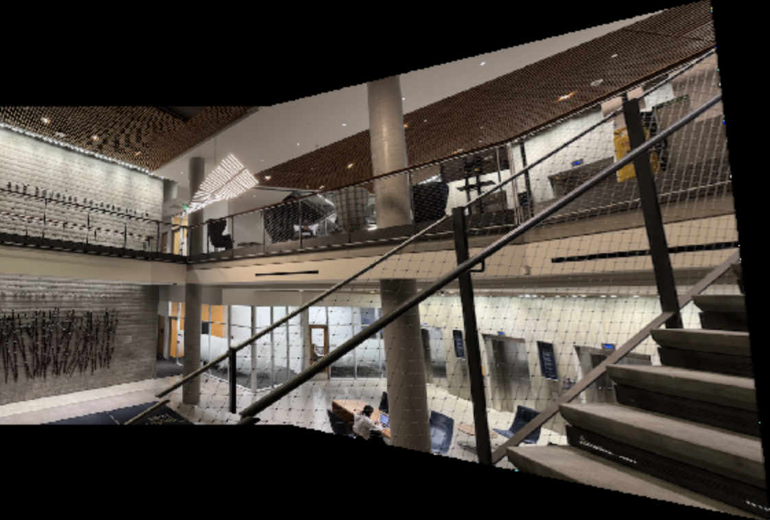
Here is an example of a failure case. I believe the railing in the forefront of the image is difficult to align whereas the background is well- aligned. Maybe using a spherical warp or using more correspondence points can help tackle this so that the features at the very front are also aligned.
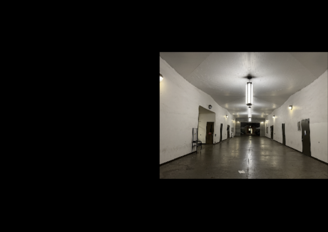
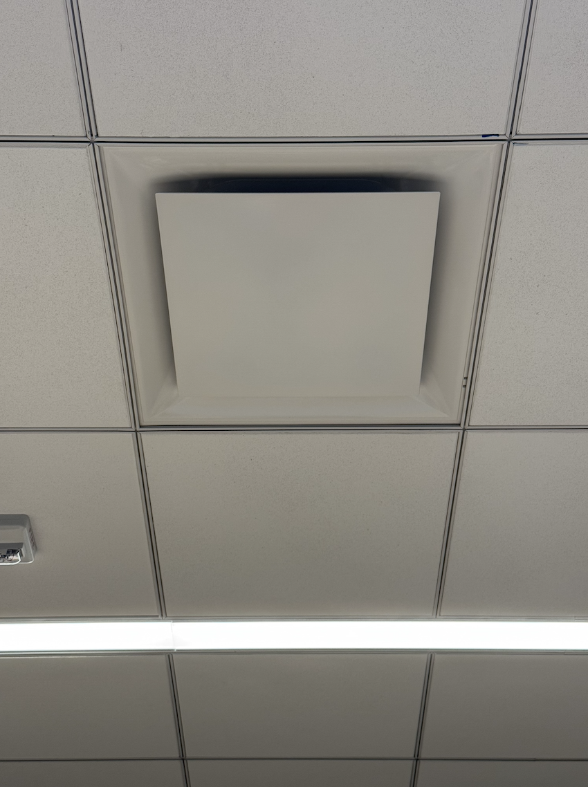
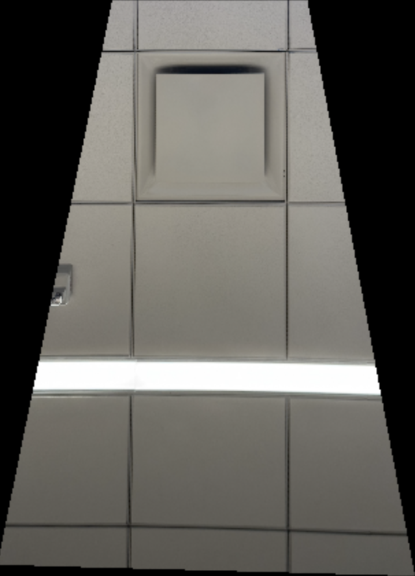
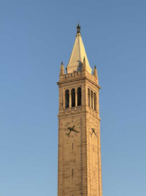
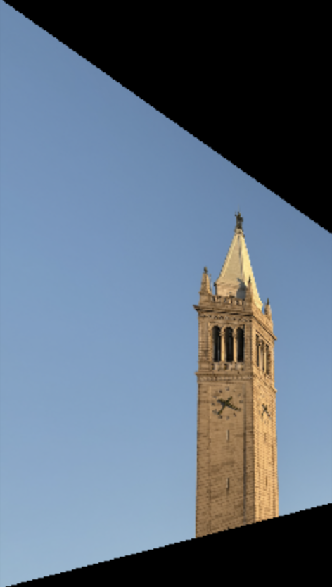
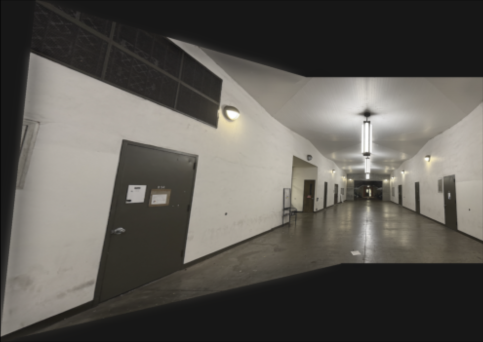
To ensure that my homography and warping is working correctly, I performed image rectification. I took pictures of things that I knew were square at an angle so that they weren't square in the image. I then rectified the images by warping the images so that the features become square. First, using the online tool, I selected four points in the original image that would map to a square, which I defined manually, and then I compute the H matrix using these correspondence points. Using this H matrix, we warp the image so that the features become square. The black areas of the image are caused due to the distortion of perspective. For the moffitt ceiling, I chose four corners of one tile on the ceiling to rectify and as you can see all the tiles in the rectified image are now square. For the campanile, I chose the four corners around the clock face and as you can see, the bounding box around the clock face has become a square. Here are the images before and after rectification:
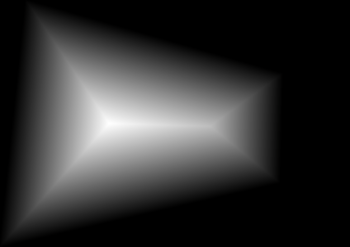
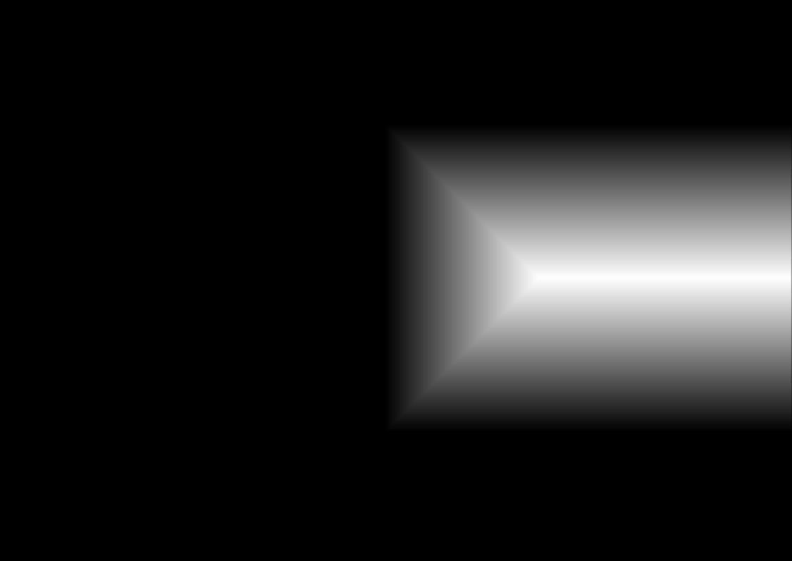
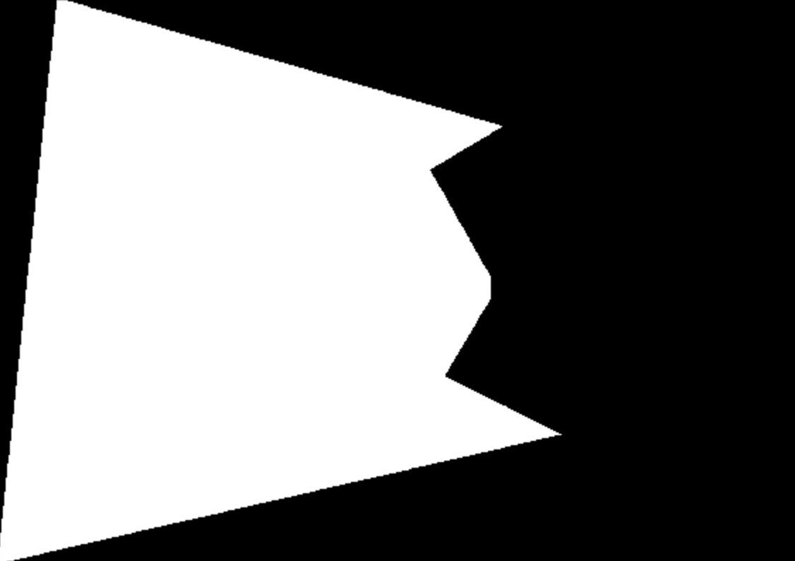
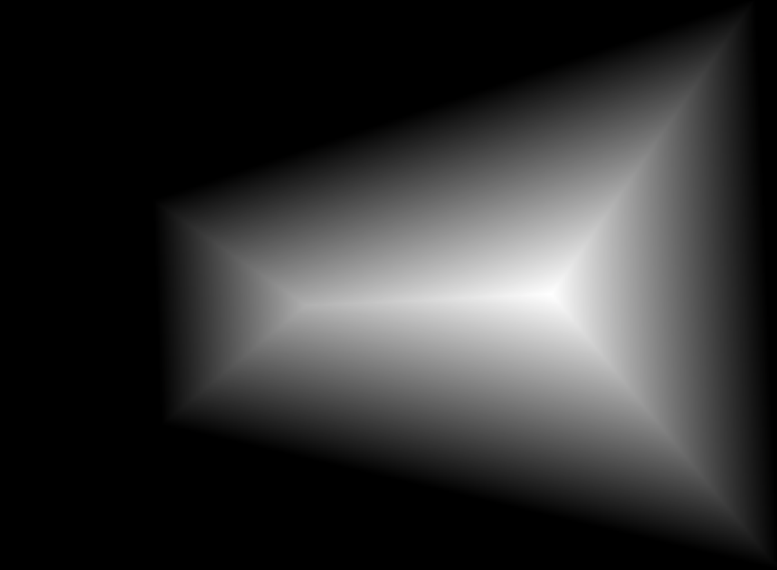
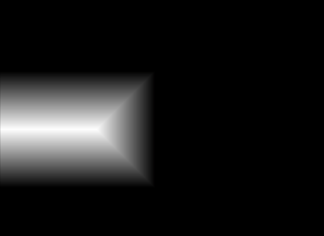
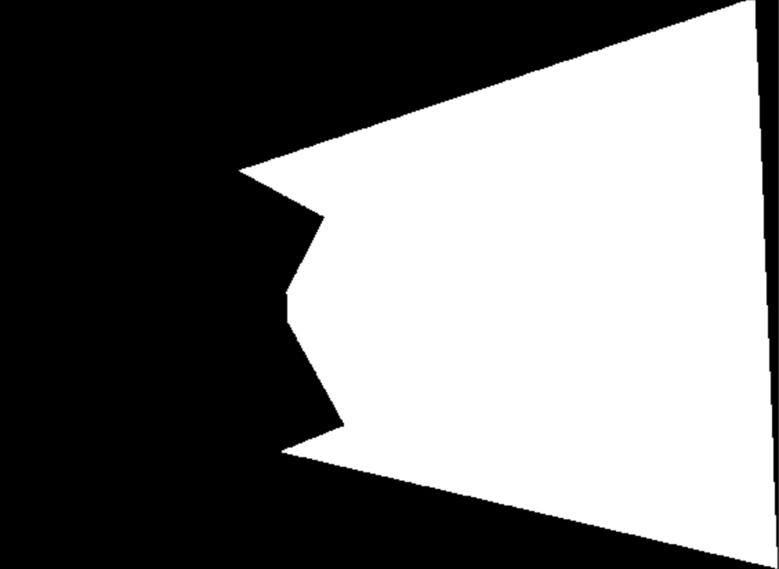
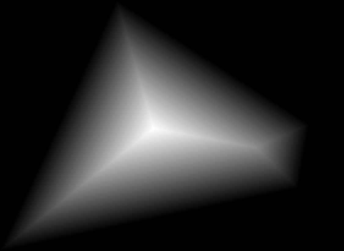
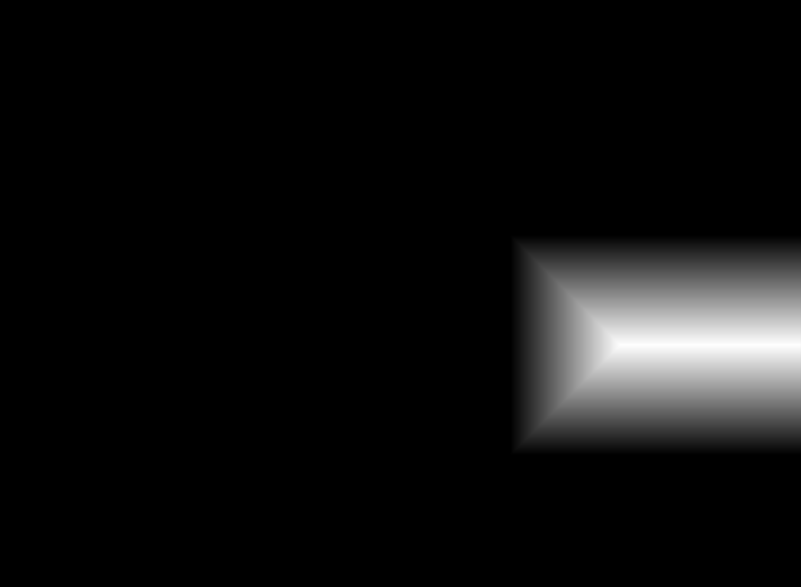
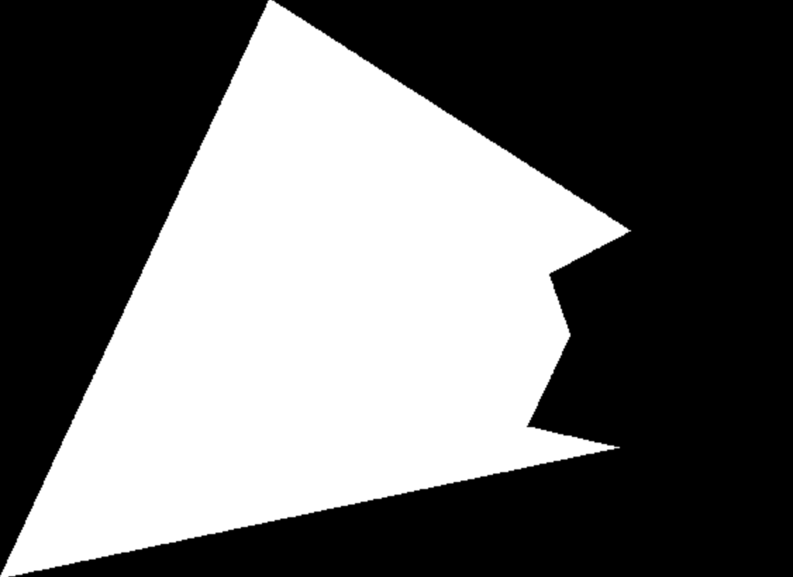
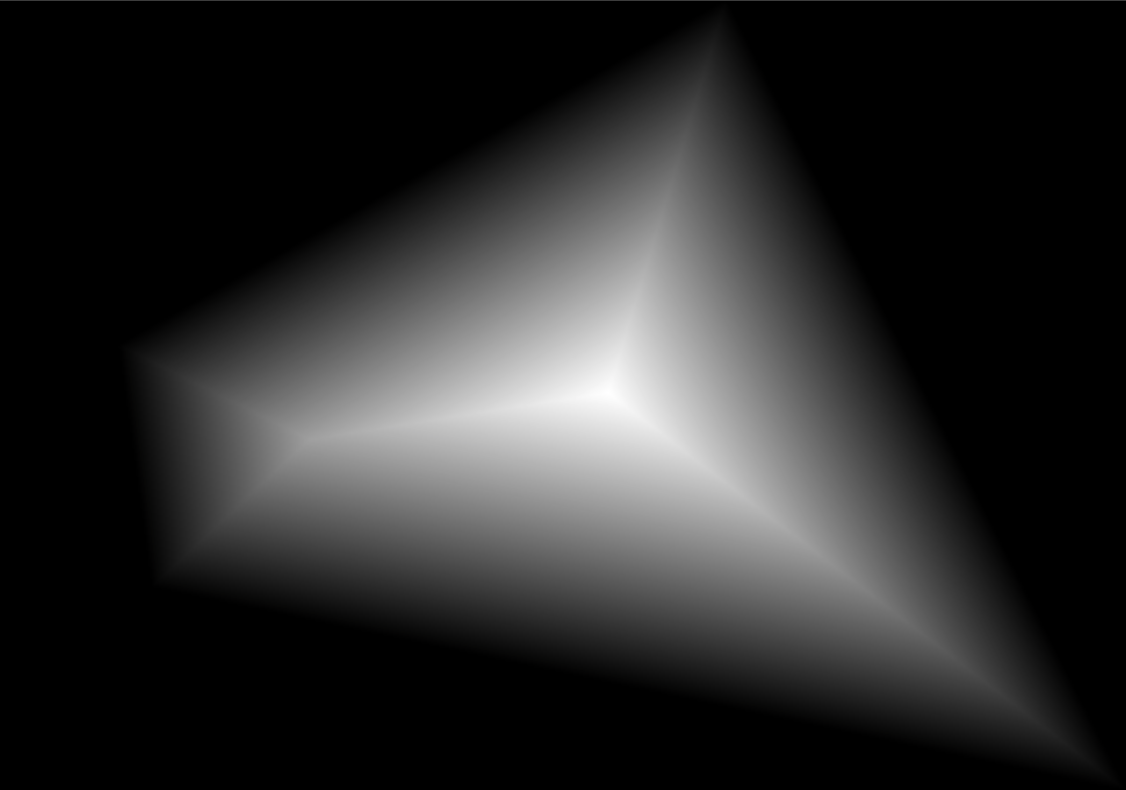
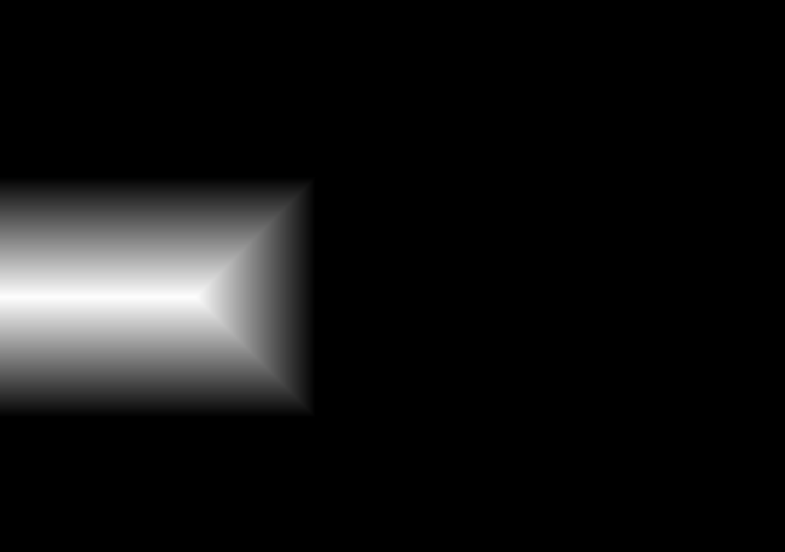
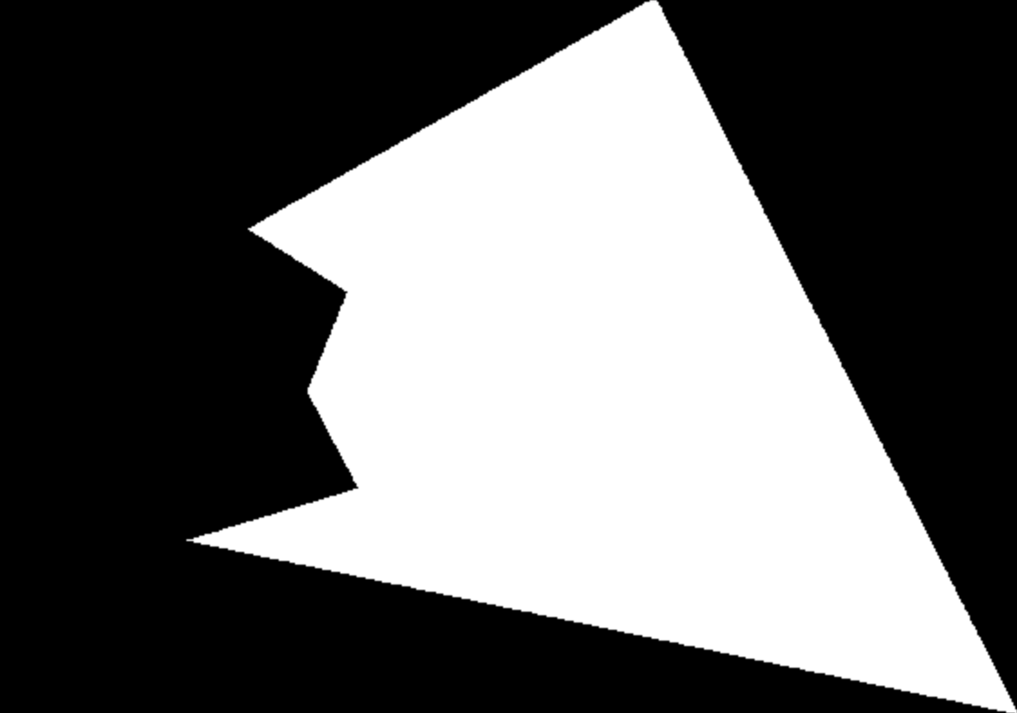
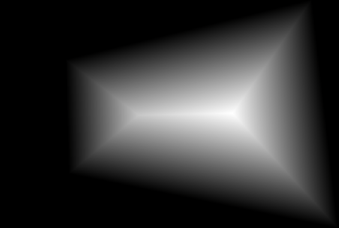
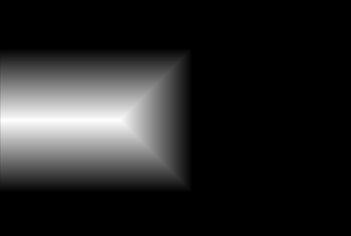
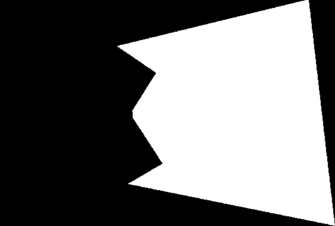
After we checked that the warping works as expected, I proceeded to blend the images seamlessly so that it looks like one image. I do this by first finding the distance transforms for the warped image and the reference image. These distance transforms are calculated by assigning each pixel in the region the distance to the nearest edge. The final result is then normalized to get a mask with values ranging from 0 to 1. Below I have shown the visualizations of these distance transforms. I then created a mask such that a pixel's value in the warped image will be taken if its distance transform in the warped image is larger than its distance transform in the reference image. Using this mask, the warped image and the reference image in the warped bounding box, I constructed Gaussian and Laplacian stacks similar to Project 2 and blended the two images together seamlessly to produce the final blended outputs which you see below:
Even when blended, the misalignment of the railing is too obvious whereas the background seamlessly blends together:
In part B of this project, we create a system for automatically stitching images into a mosaic by learning how to read and implement the research paper found at this link: https://inst.eecs.berkeley.edu/~cs180/fa24/hw/proj4/Papers/MOPS.pdf.
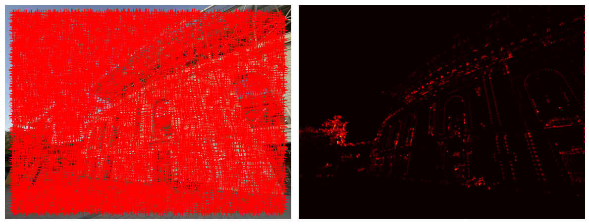
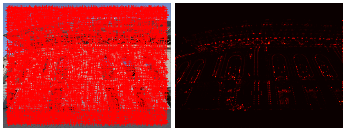
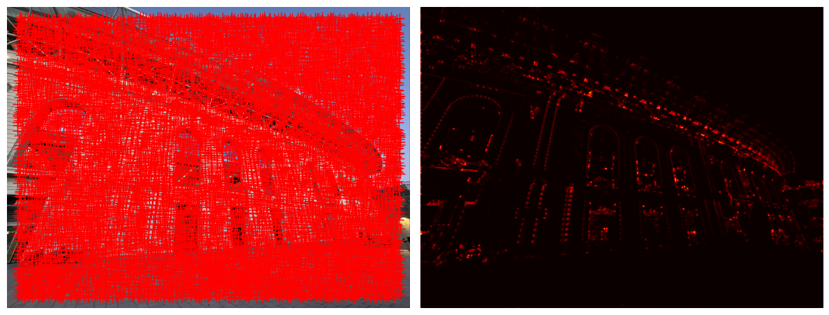
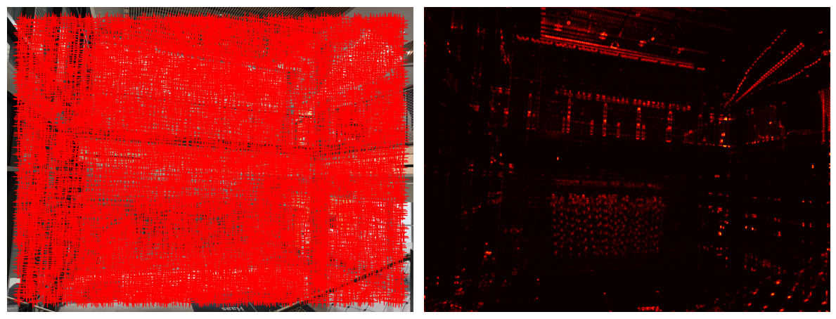
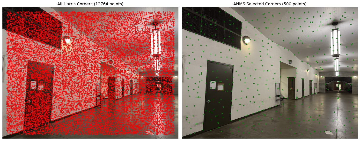
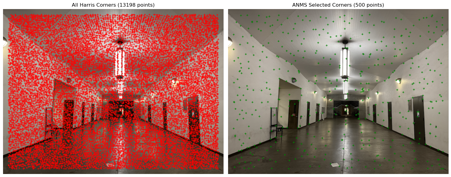
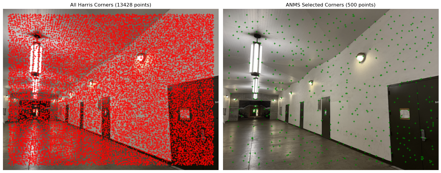
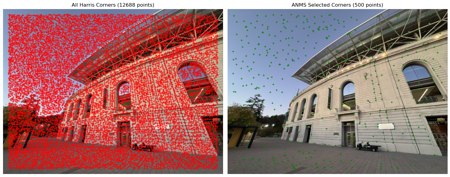
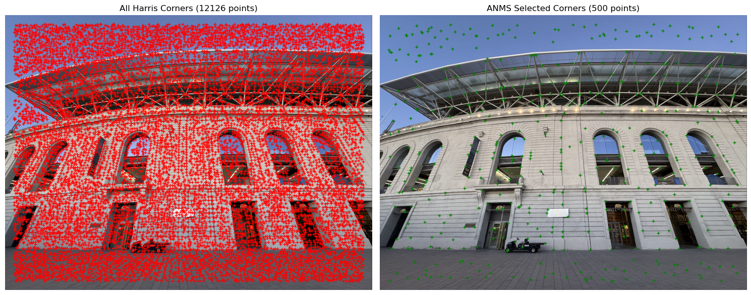
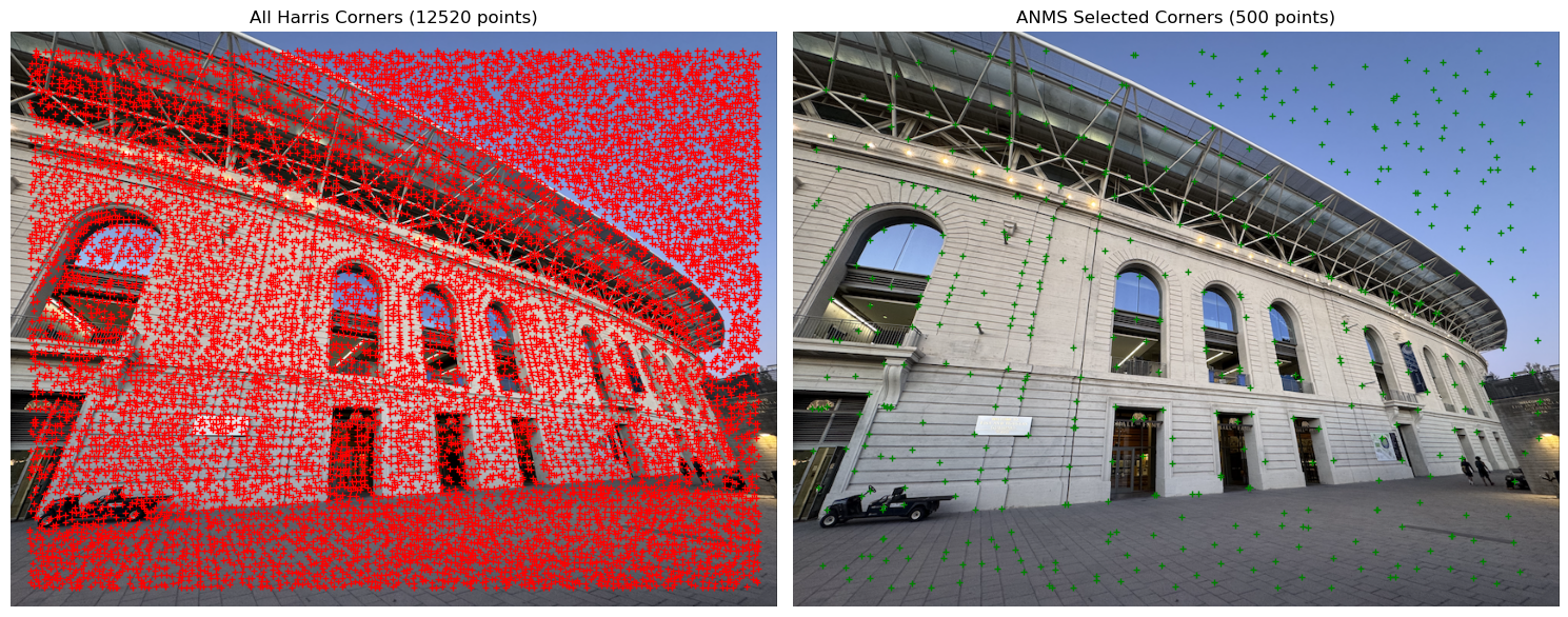
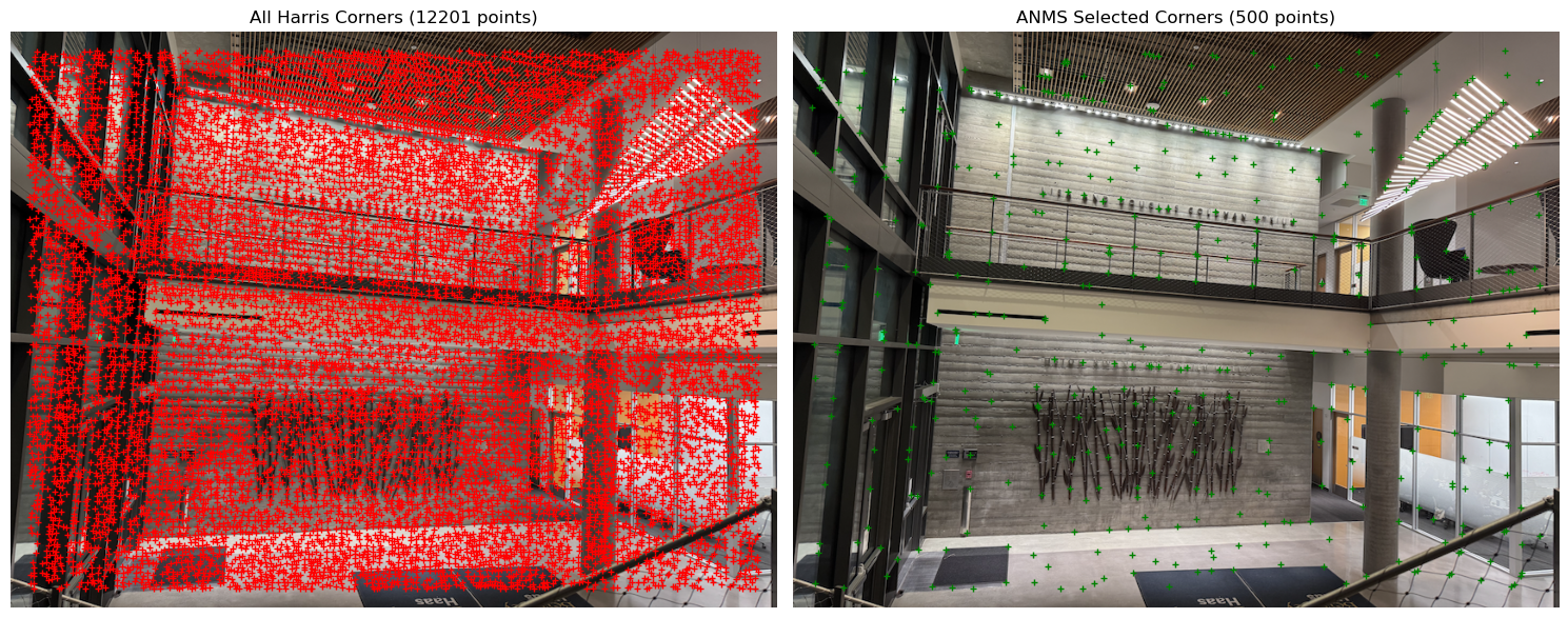
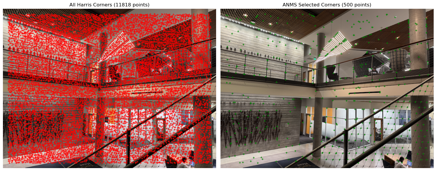
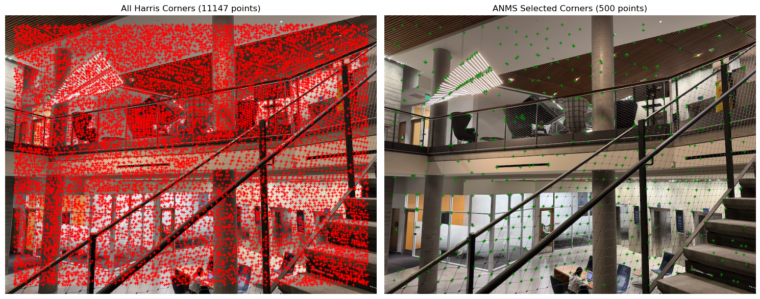
First, in order to detect the features, we need to identify the corners first because they are localized, distinct and can be found in two images of the same scene. These are great properties of corners that will be useful later on in the project. As a result, I used the corner_harris function from the skimage.feature library to find all the Harris corners in the image. Once I found them, I plotted them on the images as you can see below.
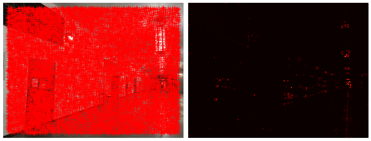
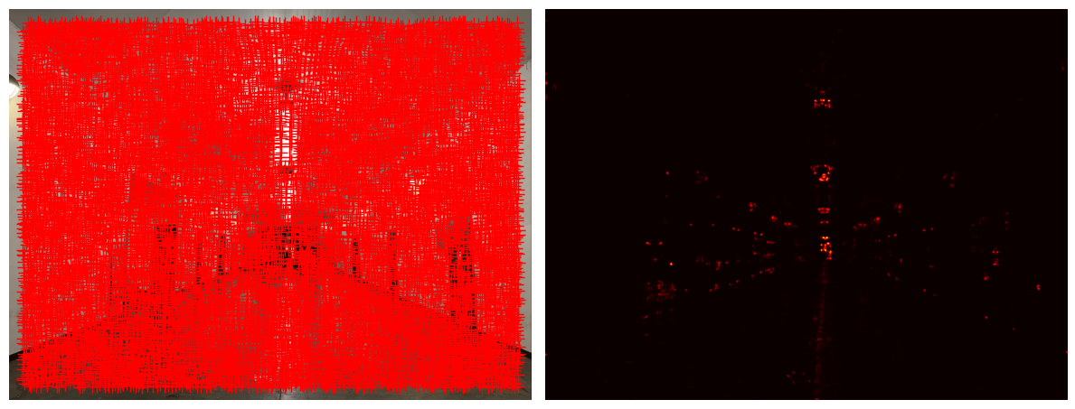
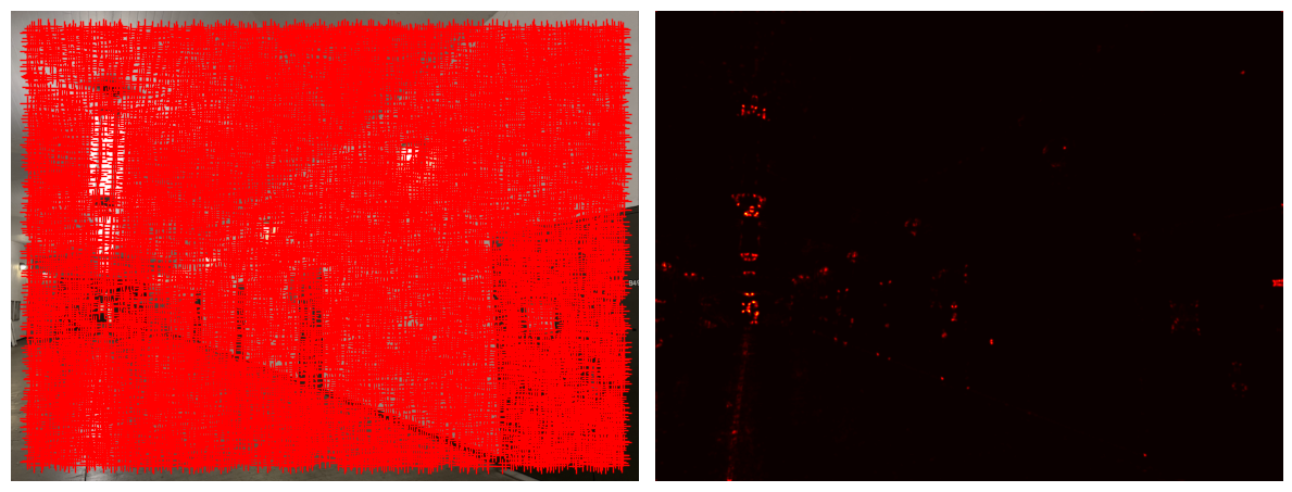
ANMS helps distribute feature points more evenly across the image instead of clustering them in highly textured areas like with the Harris Corners. For image stitching, we need good feature matches across the entire overlap region between images, not just in small clustered areas. In terms of implementation, I only keep the points that have a longer distance to strong corner intensities, which allows the points to be evenly distributed. For each point, I find the minimum distance to any other point that is stronger than the threshold, which is the suppression radii. I then sort each point by their suppression radii in descending order from largest to smallest and keep the top 500 points. Below, you can see the selected points overlaying the respective image.
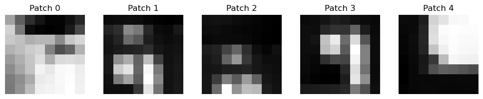
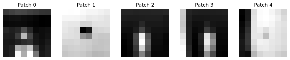
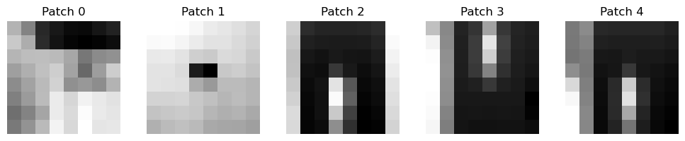
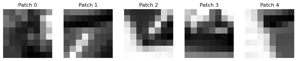
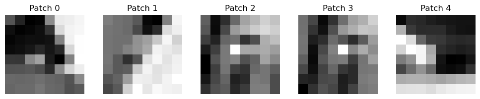
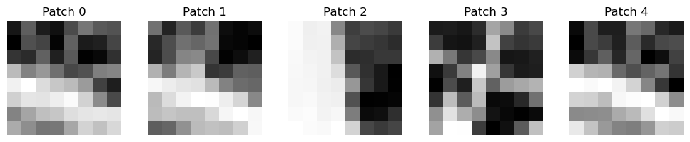
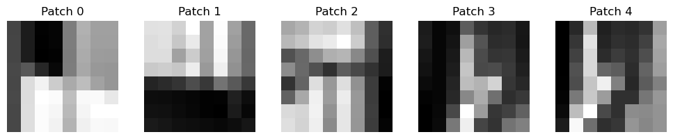
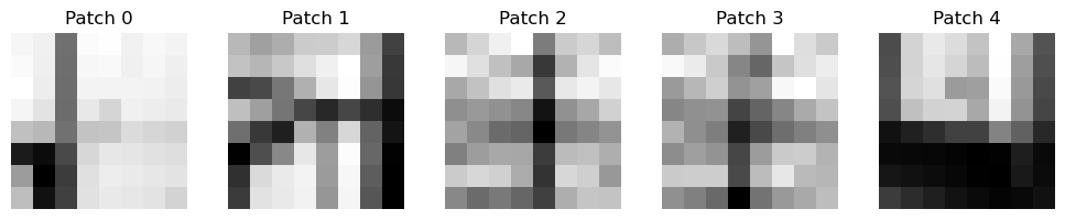
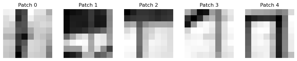
The feature descriptor extraction is necessary for creating distinctive 8x8 windows of each feature point. By first extracting a 40x40 window around each corner and downsampling it to 8x8, we naturally blur it to make the descriptor more robust to small pixel variations and noise. Additionally, the bias/gain normalization step ((patch - mean)/(std)) ensures the descriptor is not affected by lighting differences so therefore we can match features even when one image is brighter or darker than the other. These normalized 8x8 patches are great, reliable descriptors to help us match corresponding points between images, making the matching process much more efficient than using raw pixel values.
For feature matching, I find the corresponding points between two images by comparing their feature descriptors which we computed in the previous section. For each descriptor in the first image, it computes the Euclidean distances to all the descriptors in the second image, which creates a distance matrix. I wrote a fidn2nn function which helps find the two nearest neighbours for each descriptor by keeping track of the two smallest distances and their indices. I learned that the Lowe's ratio test calculates the ratio between the best and second-best match distances. If this ratio is less than 0.6, it means that the best match is significantly better than the second best, making it a good match. I used 0.6 after consulting Figure 6b in the paper. The Lowe's ratio test was necessary to effectively filter out ambiguous matches where a descriptor might be similar to various other similar regions in the other image.
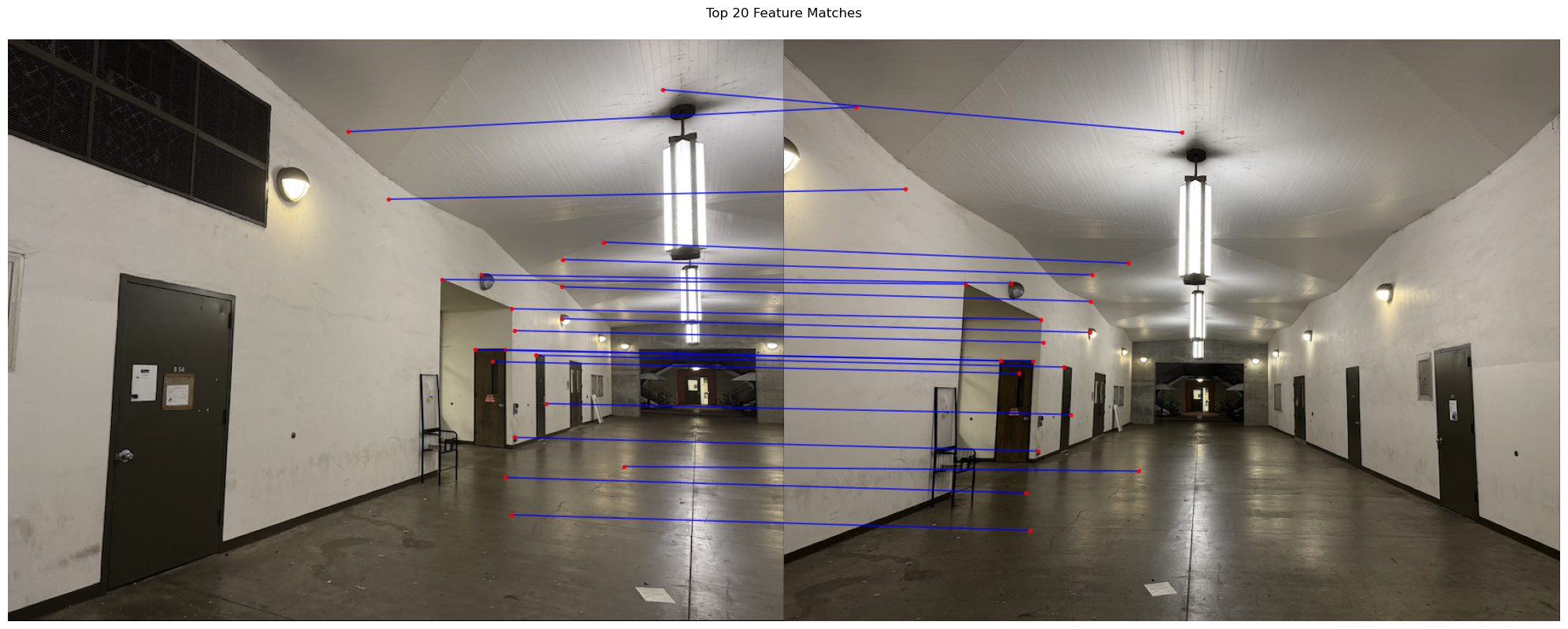
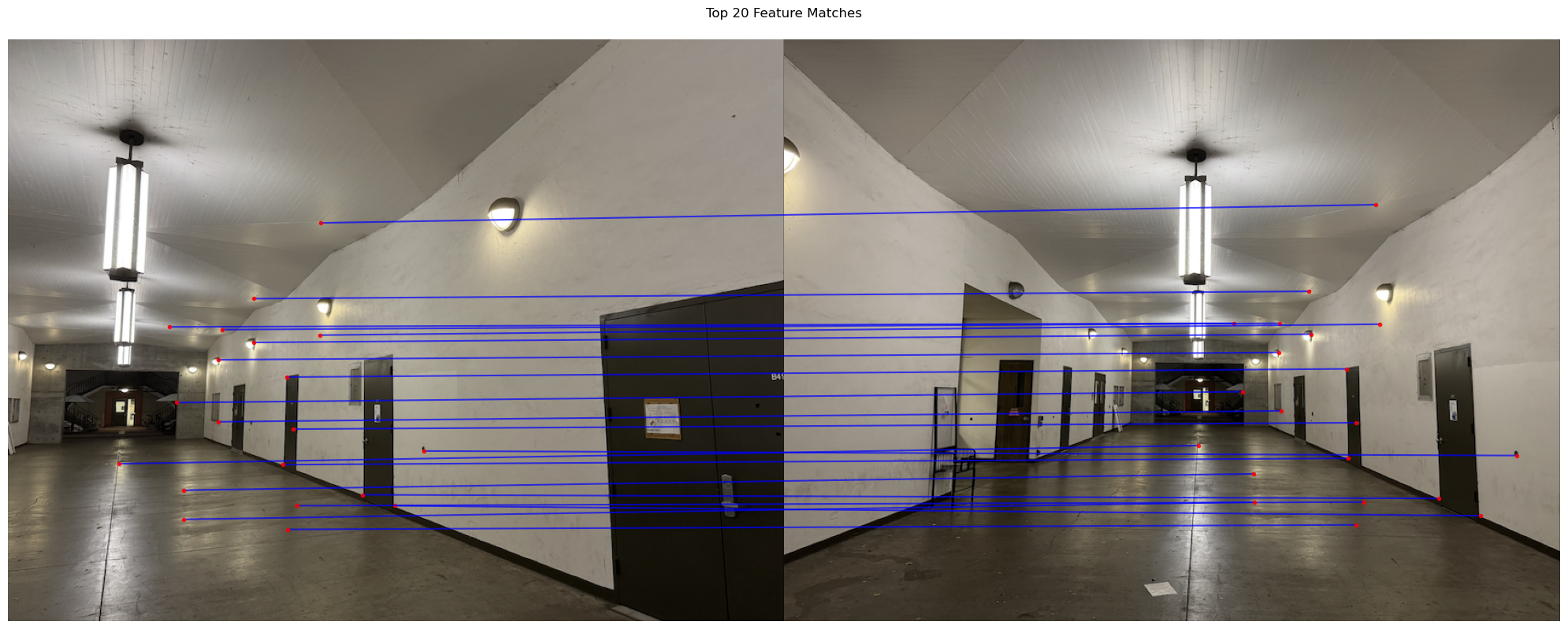
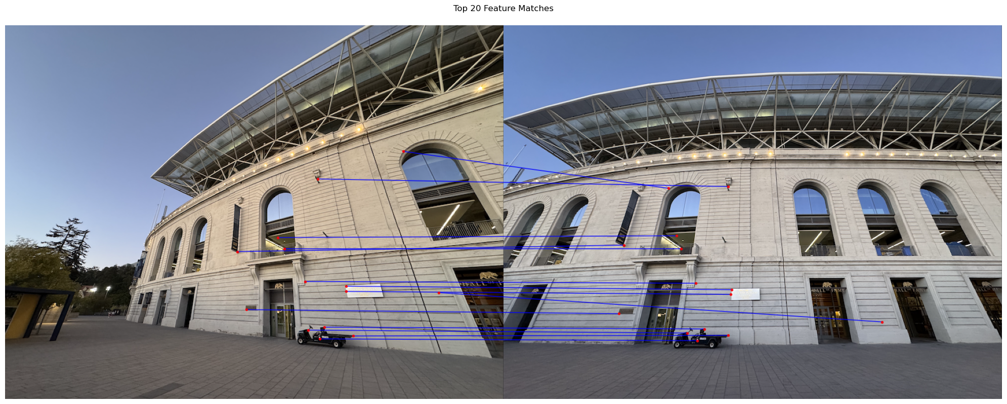
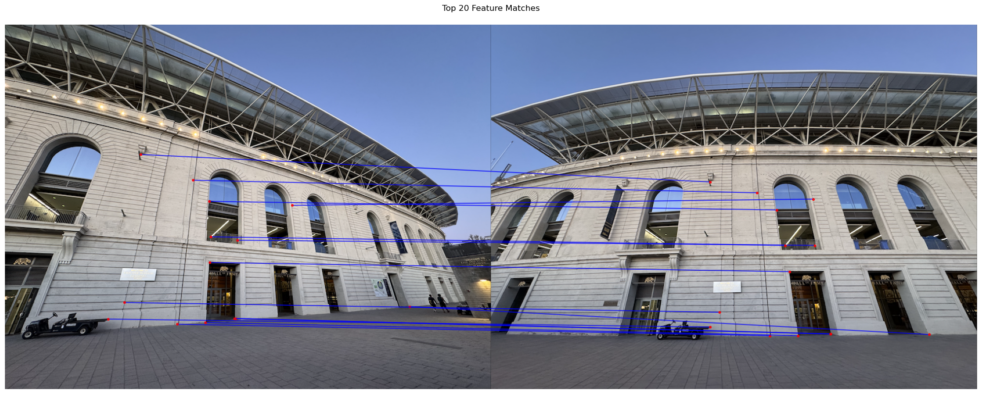
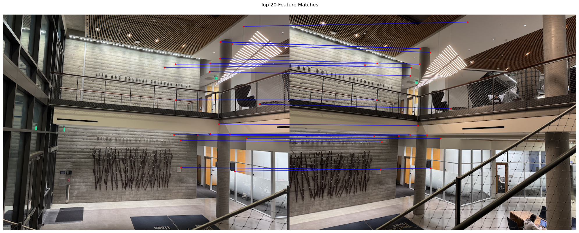
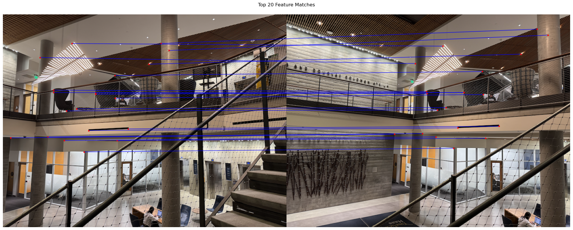
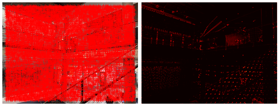
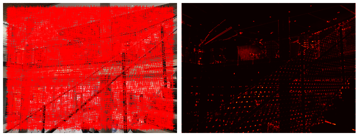
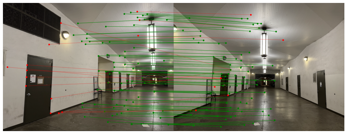
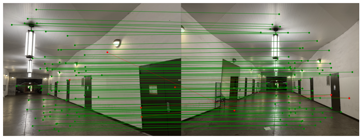
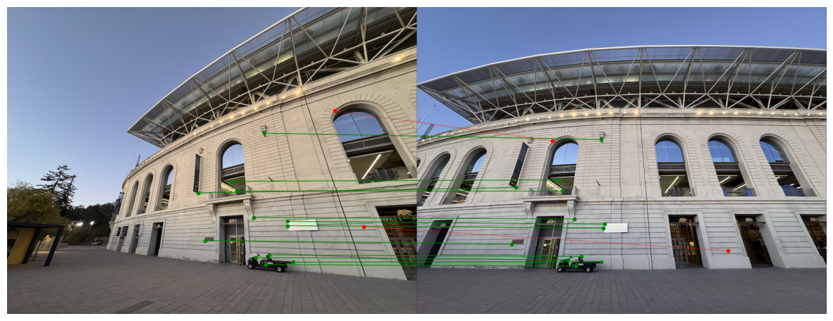
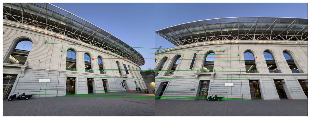
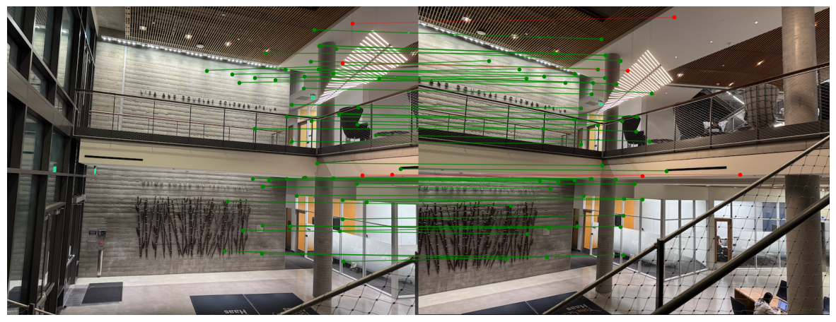
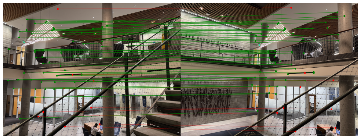
RANSAC, which stands for Random Sample Consensus, handles outliers in feature matches that could severely affect the least-squares solution. To write the RANSAC algorithm, I followed the RANSAC loop taught in lecture. Instead of using all of the matches to compute the homography, RANSAC repeatedly samples small random sets of four point pairs, computes a homography from each sample, and counts how many other points agree with this transformation (inliers). Once I computed all the inliers, I kept the largest set of inliers and recomputed the least-squares homography estimate, ransac_H, on all the inliers. RANSAC helps increase the robustness of least-squares when finding the homography matrix necessary for image stitching in the next and final step. Below are some images with the inliers overlaid:
Using the homography matrix produced by the RANSAC algorithm, I recovered the homographies and repeated the steps in part A to warp image 1 onto image 2 and blend the two images together into a smooth mosaic. Below are the final results of the automatic stitching beside the results of the manual stitching.
The coolest thing I have learned in this project is feature matching through automatic correspondences. I find it fascinating how we can create feature descriptors to help us uniquely identify a feature in one image that can be compared with other feature descriptors in other images to match the features efficiently. It is so much faster and produces better outputs than manual correspondences.