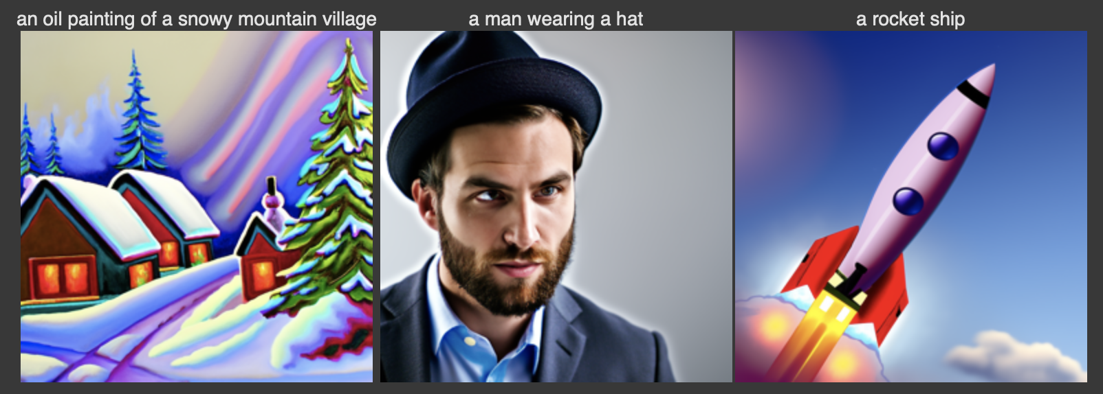
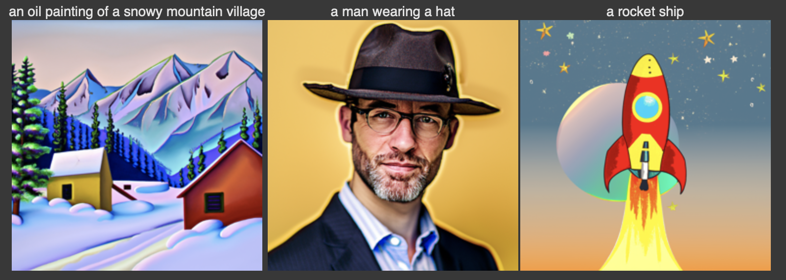
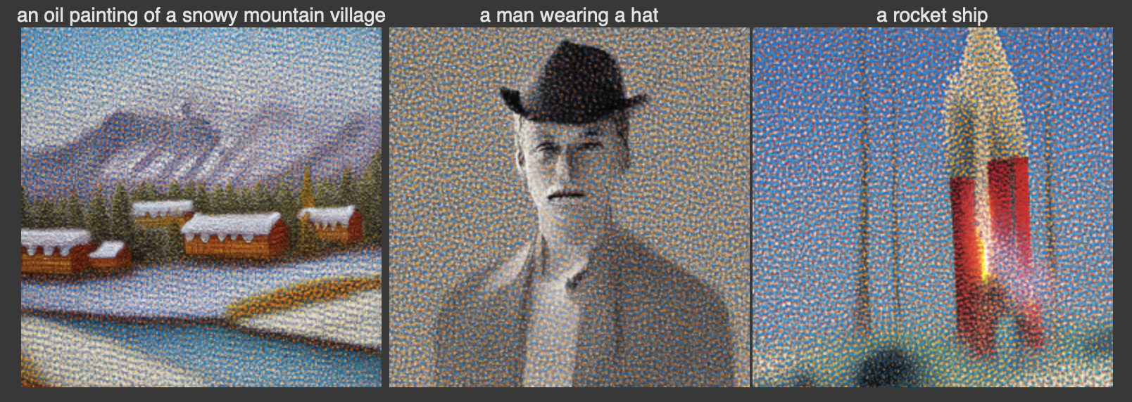
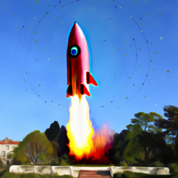
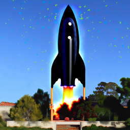
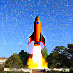
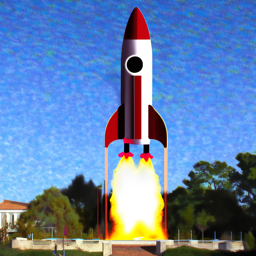
For this project, I am going to use the DeepFloyd IF diffusion model. DeepFloyd is a two stage model trained by Stability AI. The first stage produces images of size 64 x 64 and the second stage takes the outputs of the first stage and generates images of size 256 x 256. DeepFloyd was trained as a text-to-image model, which takes text prompts as input and outputs images that are aligned with the text. Because the text encoder is very large, and barely fits on a free tier Colab GPU, I precomputed a couple of text embeddings to try. In the notebook, I instantiate DeepFloyd's stage_1 and stage_2 objects used for generation, as well as several text prompts for sample generation. Below are three text prompts and their corresponding images. For the first one, I set the number of inference steps to 20. The images are detailed and very colourful but the definition of the images are not too sharp - it is still a little blurry. For the second one, I increased the number of inference steps to 40. The images' definition increased as the outlines of the shapes and figures are cleaner. The man wearing the hat seems more realistic than the previous set of images whereas the rocket ship seems more like a 2D cartoon. For the third one, I decreased the number of inference steps to 5. The quality of the images decreased by a lot and the colours are very dull and muted. The images are not as clear as the previous sets of images and there is some speckling across the images which makes it harder to see the key features in the image. The objects in the image seem to be represented more abstractly and less realistically. Therefore, increasing the number of inference steps produces more detailed, bright and realistic images whereas decreasing the number of inference steps produces more abstract, dull, and less detailed images. I am using the seed = 180.

A key part of diffusion is the forward process, which takes a clean image and adds noise to it. In this part, I write a function to implement this. Given a clean image, we get a noisy image at timestep t by sampling from a Gaussian. Note that the forward process is not just adding noise, we also scale the image.
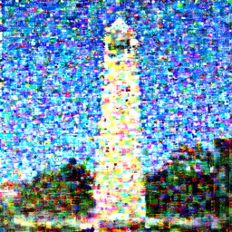
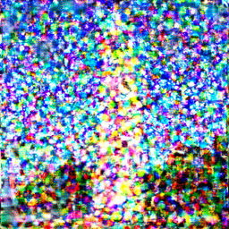
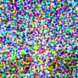
In this section, I take noisy images for timesteps [250, 500, 750], but use Gaussian blur filtering to try to remove the noise. Getting good results was quite difficult, if not impossible.





Now, I use a pretrained diffusion model to denoise. The actual denoiser is stage_1.unet, which is a UNet that has already been trained on a very, very large dataset of pairs of images. We can use it to recover Gaussian noise from the image. Then, we can remove this noise to recover something close to the original image. Note: this UNet is conditioned on the amount of Gaussian noise by taking timestep t as additional input.
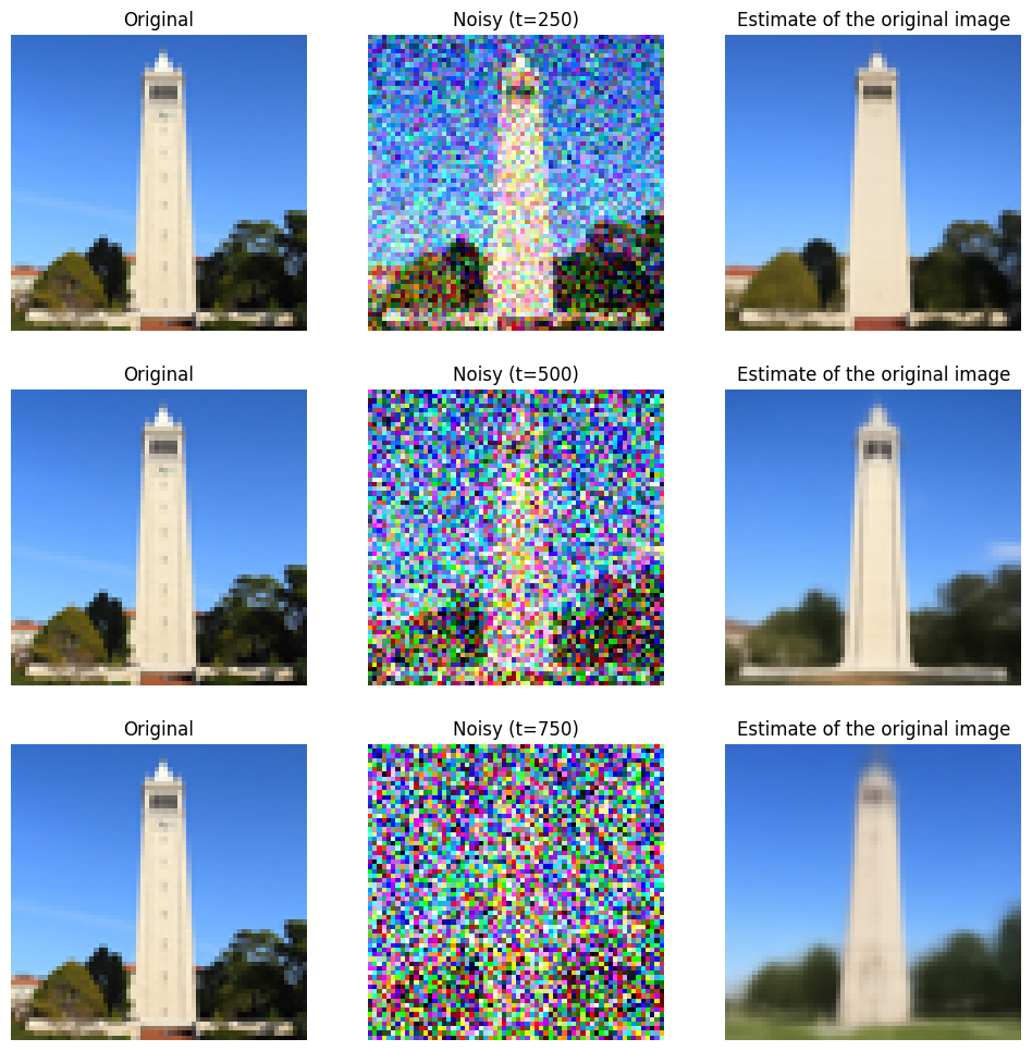
In the previous part, the denoising UNet does a much better job of projecting the image onto the natural image manifold, but it does get worse as you add more noise. This makes sense, as the problem is much harder with more noise! However, diffusion models are designed to denoise iteratively, which is what I implement in this section.
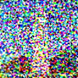
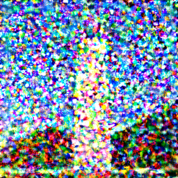
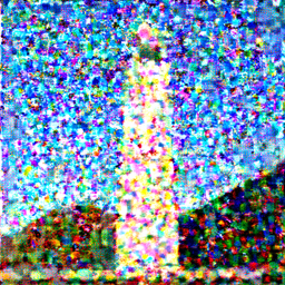
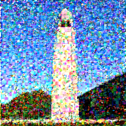
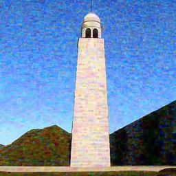
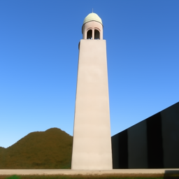
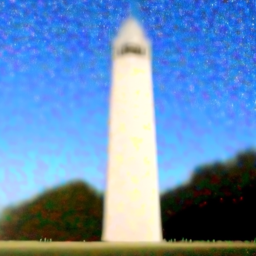
Another thing we can do with the iterative_denoise function is to generate images from scratch. We can do this by setting i_start = 0 and passing in random noise. This effectively denoises pure noise.
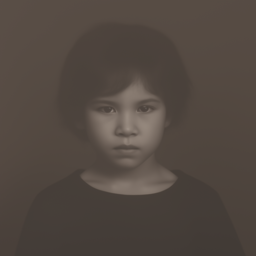
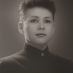
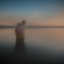
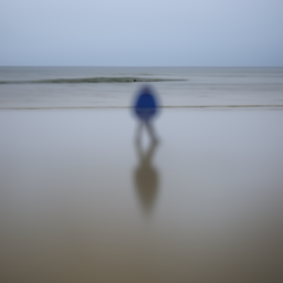
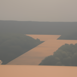
In order to greatly improve image quality (at the expense of image diversity), we can use a technique called Classifier-Free Guidance.In CFG, we compute both a conditional and an unconditional noise estimate, which we use with gamma (strength of the CFG) to calculate our new noise estimate. To get an unconditional noise estimate, we can just pass an empty prompt embedding to the diffusion model. When gamma > 1, we get much higher quality images.
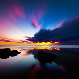
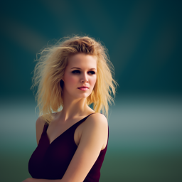
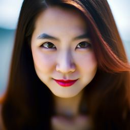
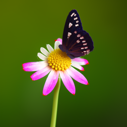
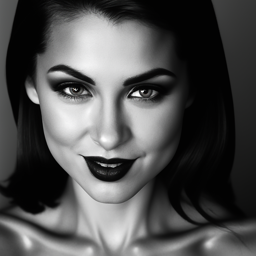
In part 1.4, we take a real image, add noise to it, and then denoise. This effectively allows us to make edits to existing images. The more noise we add, the larger the edit will be. This works because in order to denoise an image, the diffusion model must to some extent "hallucinate" new things -- the model has to be "creative." Another way to think about it is that the denoising process "forces" a noisy image back onto the manifold of natural images. Here, I am going to take the original test image, noise it a little, and force it back onto the image manifold without any conditioning. Effectively, I am going to get an image that is similar to the test image (with a low-enough noise level). This follows the SDEdit algorithm.
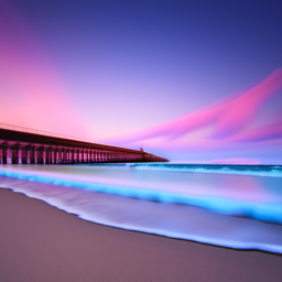
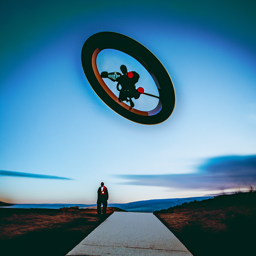
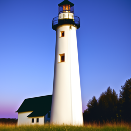
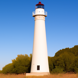
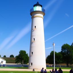
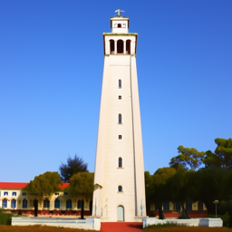
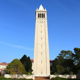
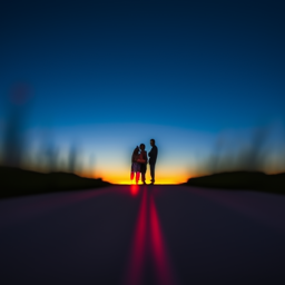
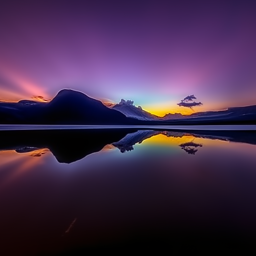
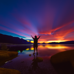
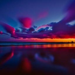
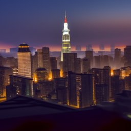
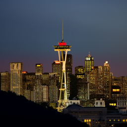
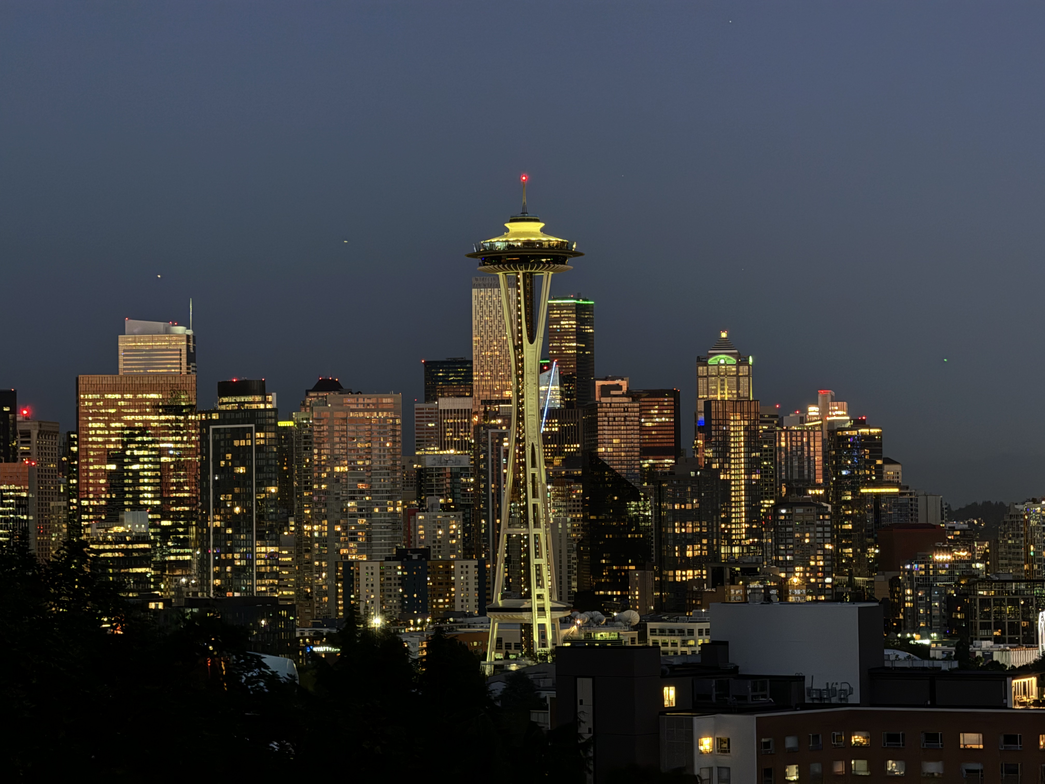
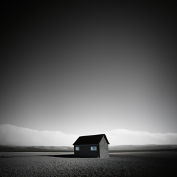
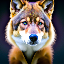
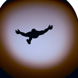
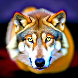
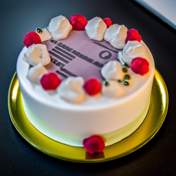

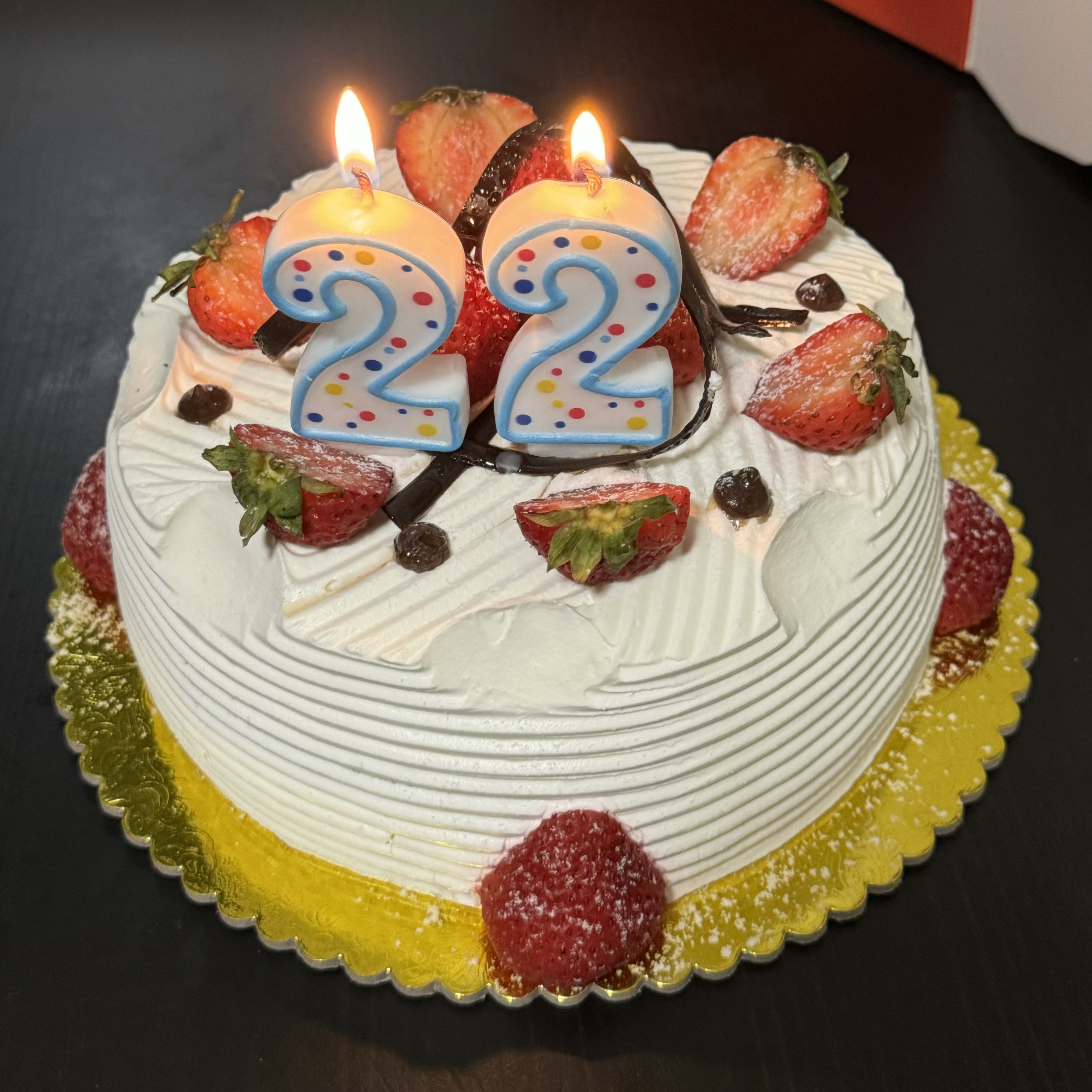
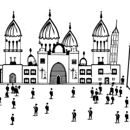
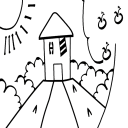
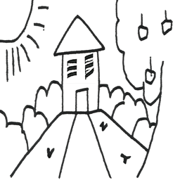
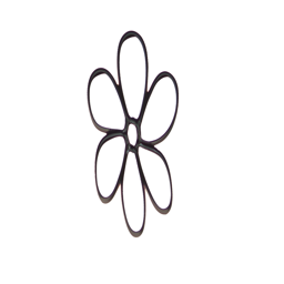
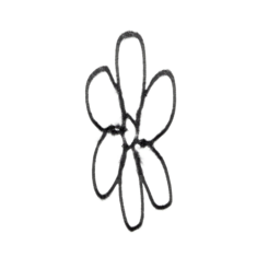
This procedure works particularly well if we start with a nonrealistic image (e.g. painting, a sketch, some scribbles) and project it onto the natural image manifold. I experiment by starting with hand-drawn or other non-realistic images and see how you can get them onto the natural image manifold in fun ways.
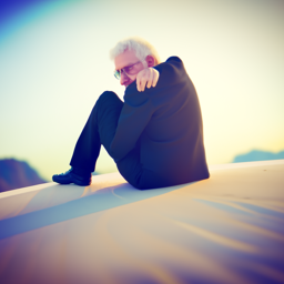
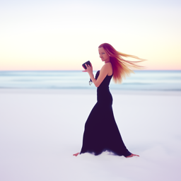
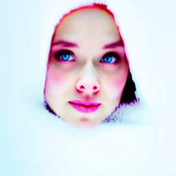




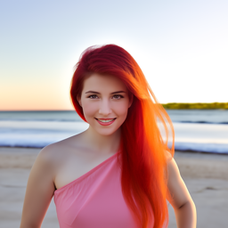
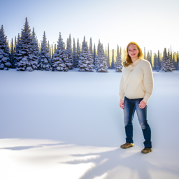
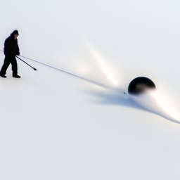

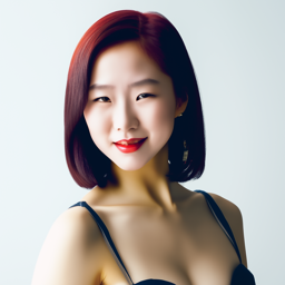
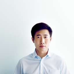
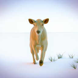


We can use the same procedure to implement inpainting (following the RePaint paper). That is, given an image, x, and a binary mask, m, we can create a new image that has the same content where m is 0, but new content wherever m is 1. To do this, we can run the diffusion denoising loop. But at every step, after obtaining the image, we "force" it to have the same pixels as the original images, where m is 0. Essentially, we leave everything inside the edit mask alone, but we replace everything outside the edit mask with our original image - with the correct amount of noise added for timestep, t.
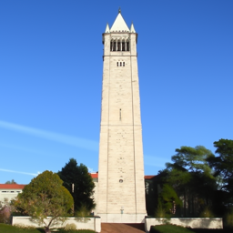
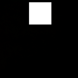
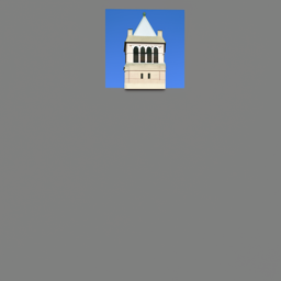
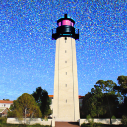
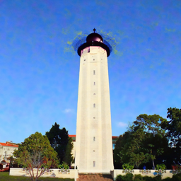
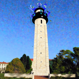
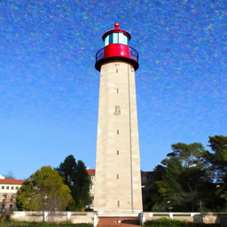
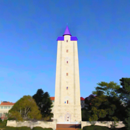
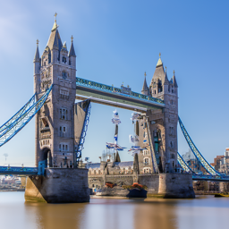

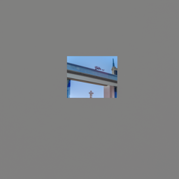
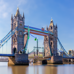
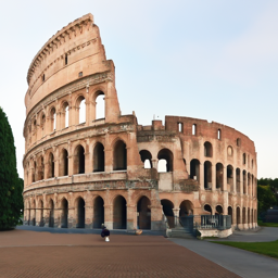

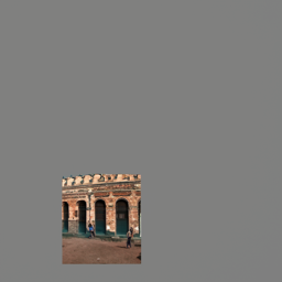
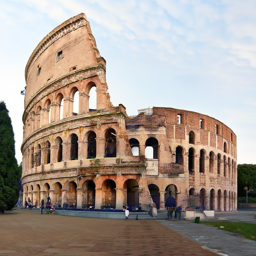
Now, we will do the same thing as SDEdit, but guide the projection with a text prompt. This is no longer pure "projection to the natural image manifold" but also adds control using language.

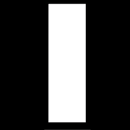
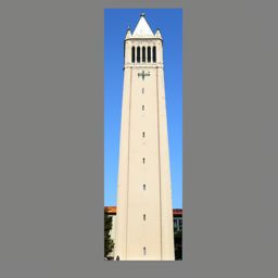
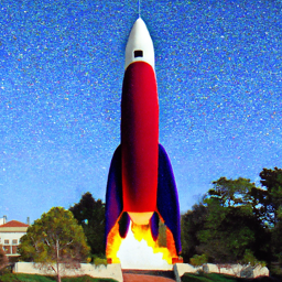
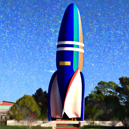

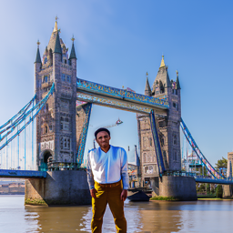
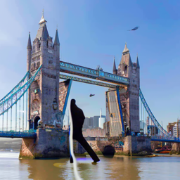
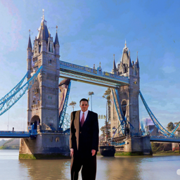
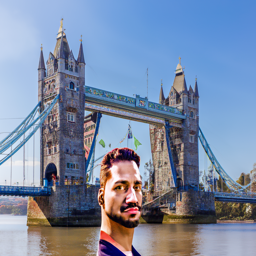
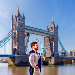
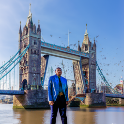
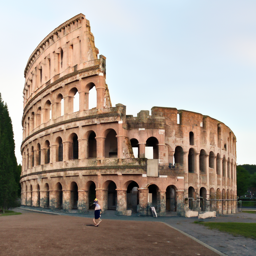
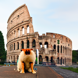
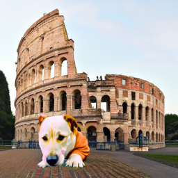
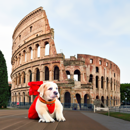
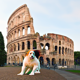
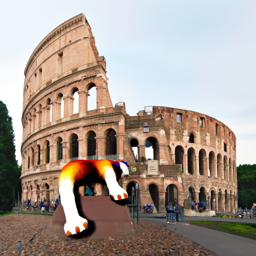
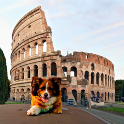
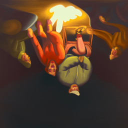
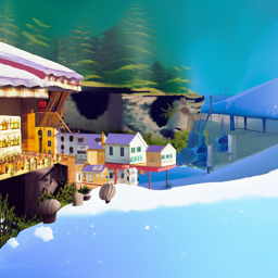
In this part, we are finally ready to implement Visual Anagrams and create optical illusions with diffusion models. In this part, I first create an image that looks like "an oil painting of people around a campfire", but when flipped upside down will reveal "an oil painting of an old man". To do this, we will denoise an image, x, at step, t, normally with the prompt "an oil painting of an old man", to obtain noise estimate e1. But at the same time, we will flip x upside down, and denoise with the prompt "an oil painting of people around a campfire", to get noise estimate e2. We can flip e2 back, to make it right-side up, and average the two noise estimates to get the final estimate. We can then perform a reverse/denoising diffusion step with the averaged noise estimate.
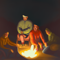
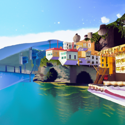

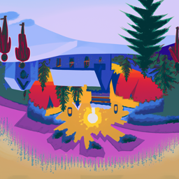
In this part we'll implement Factorized Diffusion and create hybrid images just like in project 2. In order to create hybrid images with a diffusion model we can use a similar technique as above. We will create a composite noise estimate by estimating the noise with two different text prompts, and then combining low frequencies from one noise estimate with high frequencies of the other.
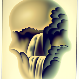
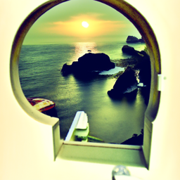
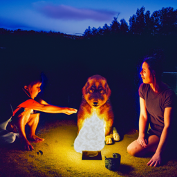
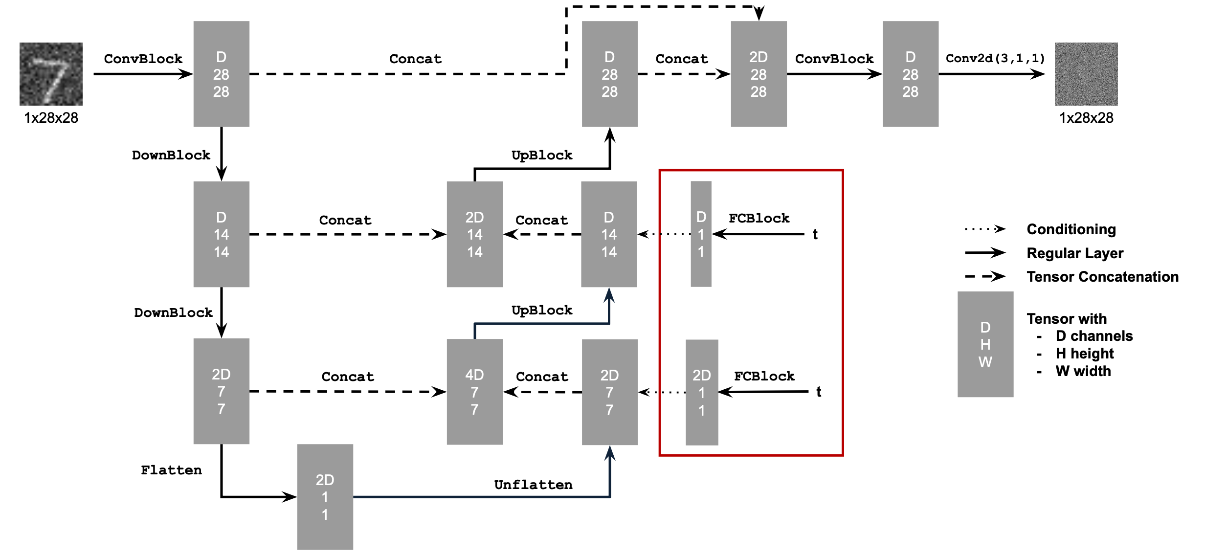
I used the below diagram to construct the various classes that I need to create the UNet:
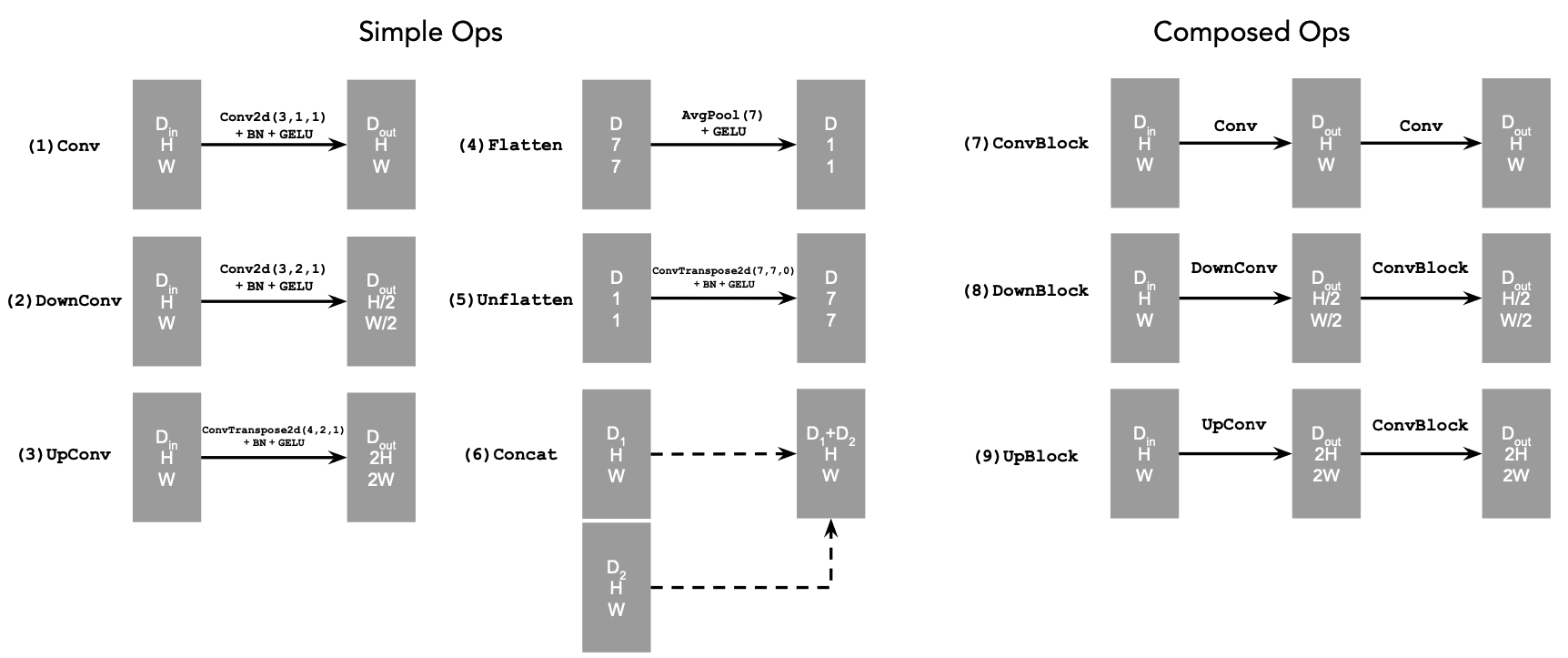
I used the below diagram to construct the UnconditionalUNet Class:

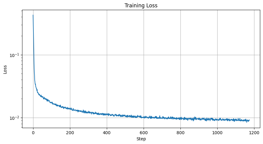
Now, we will train the model to perform denoising. The objective is to train a denoiser to denoise a noisy image, which is essentially the product of a noise level of 0.5 applied to a clean image. I use the MNIST dataset via torchvision.datasets.MNIST with flags to access both the training and test sets. Then, I train only on the training set over 5 epochs. Before I create the dataloader, I shuffle the dataset and use the recommended batch size of 256. I only noise the image batches when fetched from the dataloader so that in every epoch the network will see new noised images thus improving generalization. For the model, I use the UNet architecture previously defined with recommended hidden dimension D = 128. For the optimizer, I use the Adam optimizer with learning rate of 1e-4.
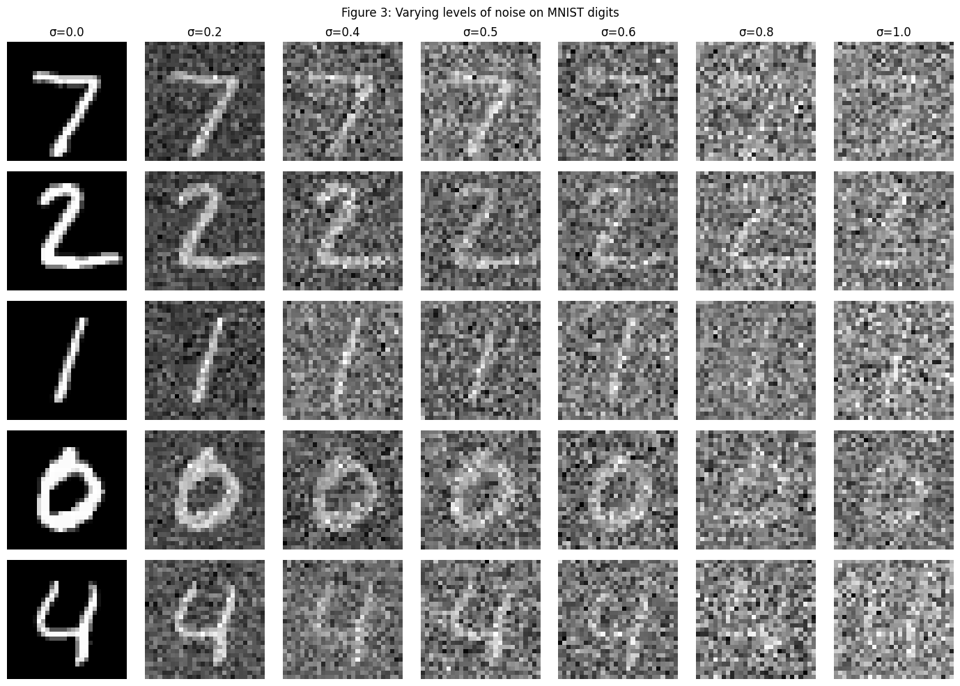
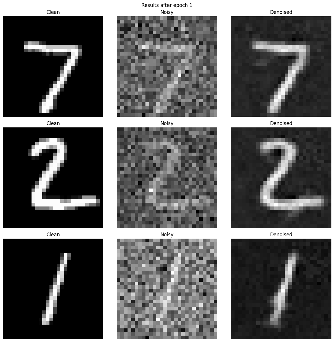
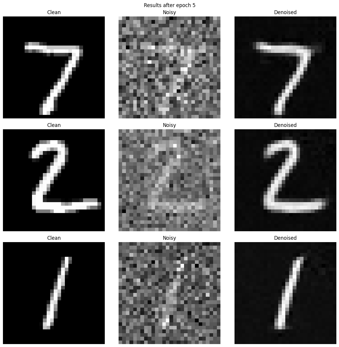
Our denoiser was trained on MNIST digits noised with noise level of 0.5. Now, let's see how the denoiser performs on different noise levels that it wasn't trained for. I visualized the denoiser results on test set digits with varying levels of noise = [0.0, 0.2, 0.4, 0.5, 0.6, 0.8, 1.0].

We need a way to inject scalar t into our UNet model to condition it. There are many ways to do this but this is how I implemented it:


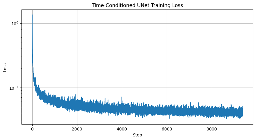
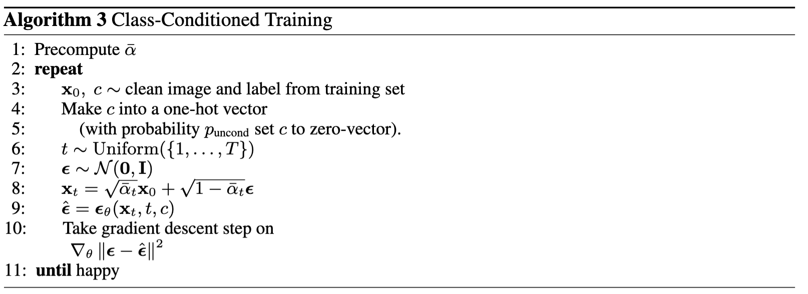
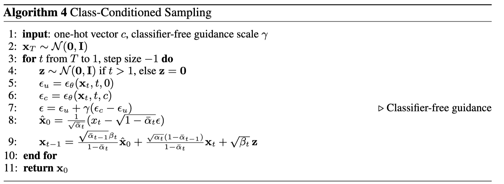
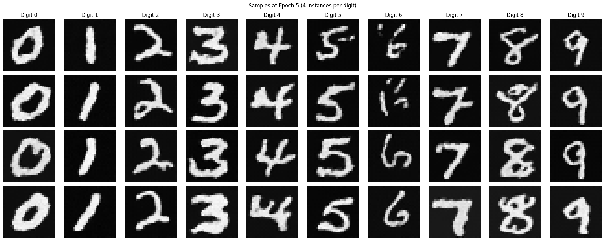
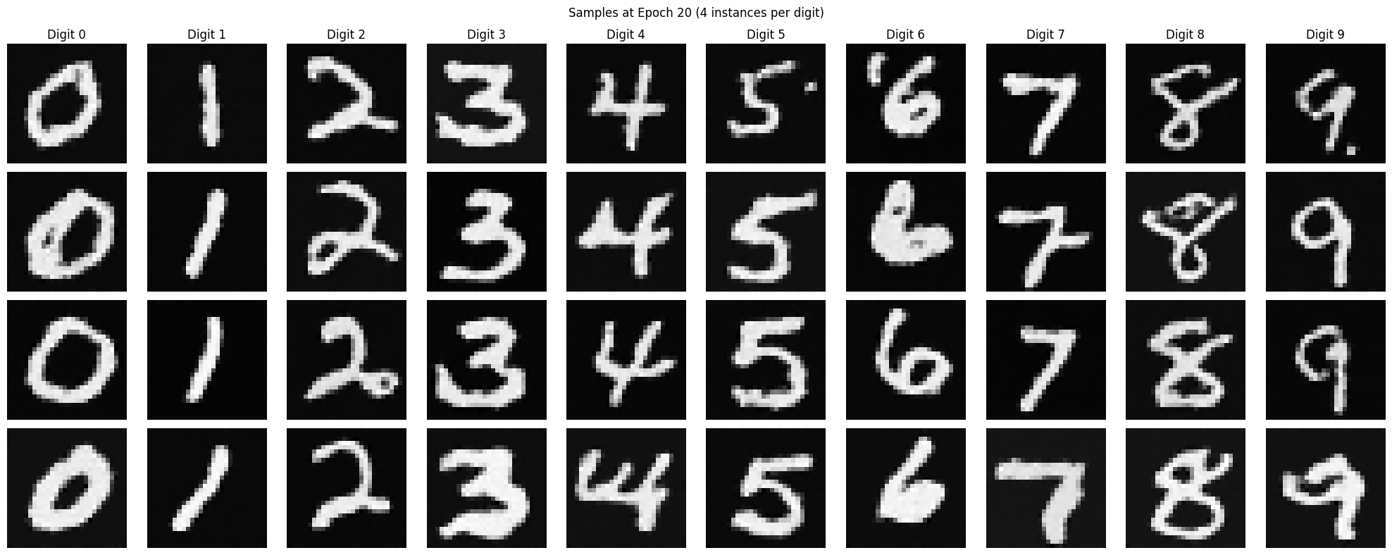
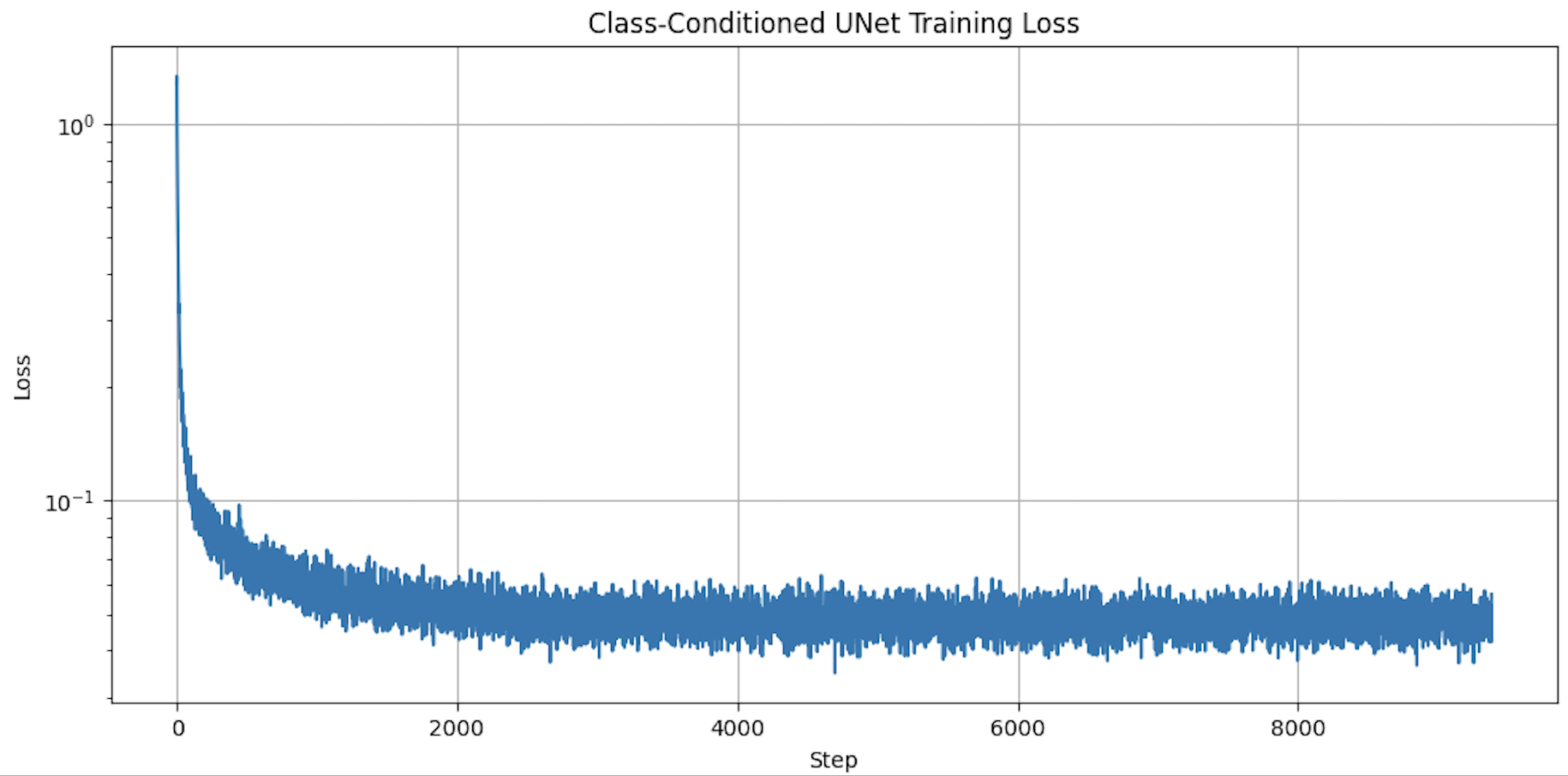
To make the results better and give us more control for image generation, we can also condition our UNet on the class of the digit 0-9. This will require adding 2 more FCBlocks to our UNet but for the class-conditioning vector, you make it a one-hot vector instead of a single scalar. Since we still want our UNet to work without it being conditioned on the class, we implement dropout where 10% of the time, we drop the class conditioning vector by setting it to 0. Training for this section will be the same as time-only, with the only difference being the conditioning vector and doing unconditional generation periodically. The sampling process is the same as part A, where we saw that conditional results aren't good unless we use classifier-free guidance so I used CFG with gamma = 5.0 for this part.
