Oriented Filters
This project revolves around re-implementing key portions of the paper "Pyramid-Based Texture Analysis/Texture". This paper uses a slightly modified laplacian pyramid, which will decompose the image into frequency bands AND orientations in the frequency domain (can imagine splitting the plotted frequency domain amplitudes into our circular frequency bands AND quadrants). By using histogram matching, we are able to generate oriented textures matching the source image. By matching histograms of not just the source and noisy images, but also the oriented laplace pyramid, we are able to generate a texture image which has actual structure to it instead of just pixels with similar values.
The goal of this project is to try and re-create the basic results of this paper in mimicing a 2D texture. I essentially implemented the algorithms described with pseudocode in the paper. If everything goes right, I will be able to showcase my ability to match textures!
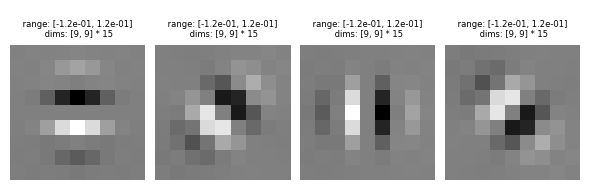
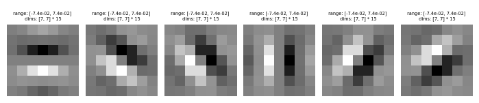
For starters, I needed to use the oriented filters talked about in the paper. In many implementations and in the steerable filters paper, the filters are defined in the frequency domain. For simplicity, we will take the approach of defining the filters in the spatial domain. To get these filters, you can use pyrtools's (a python pyramid tools library) pre-calculated oriented filters, as shown here.
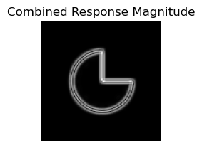
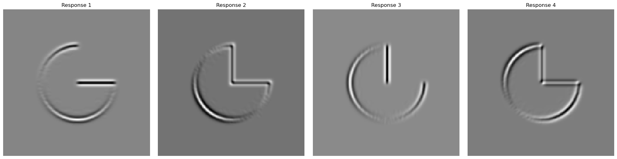
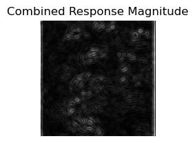
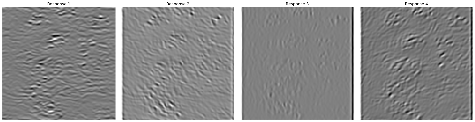
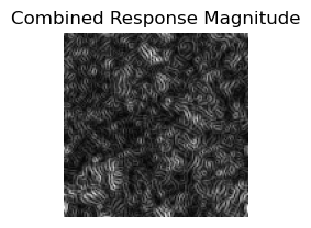
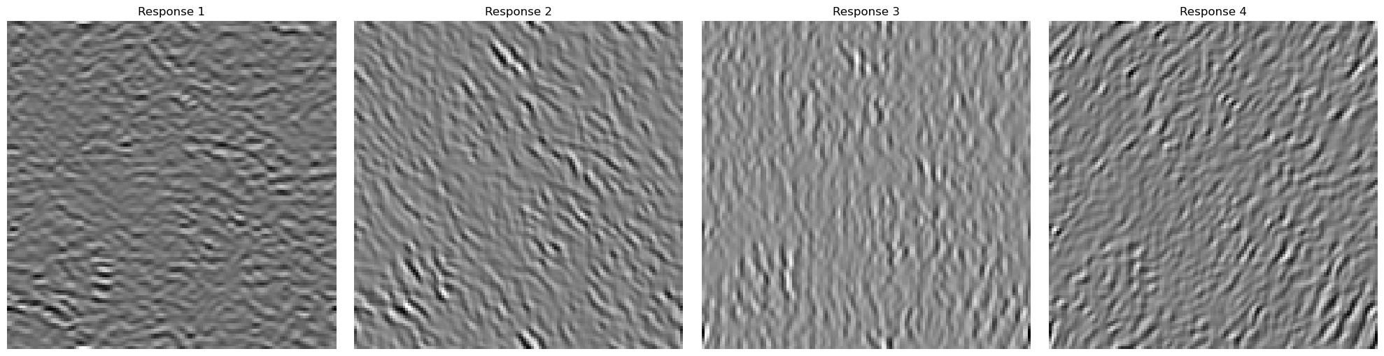
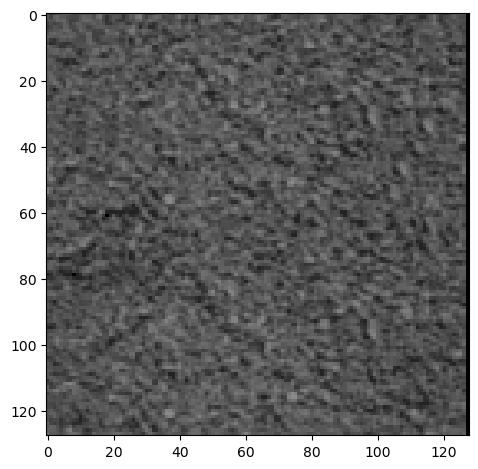
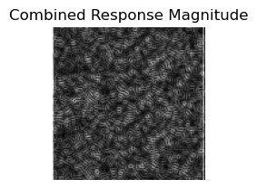
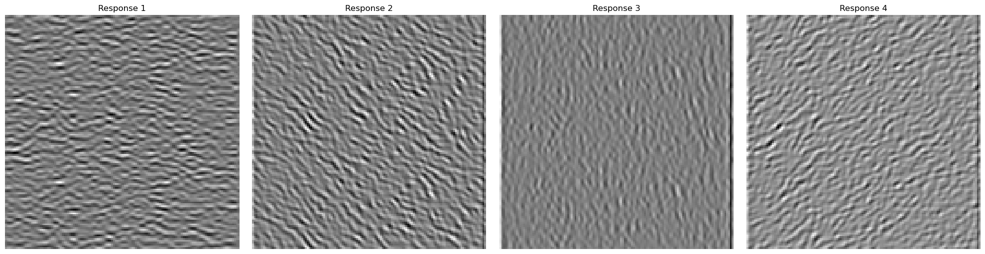
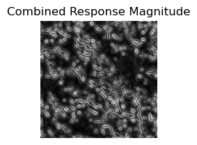
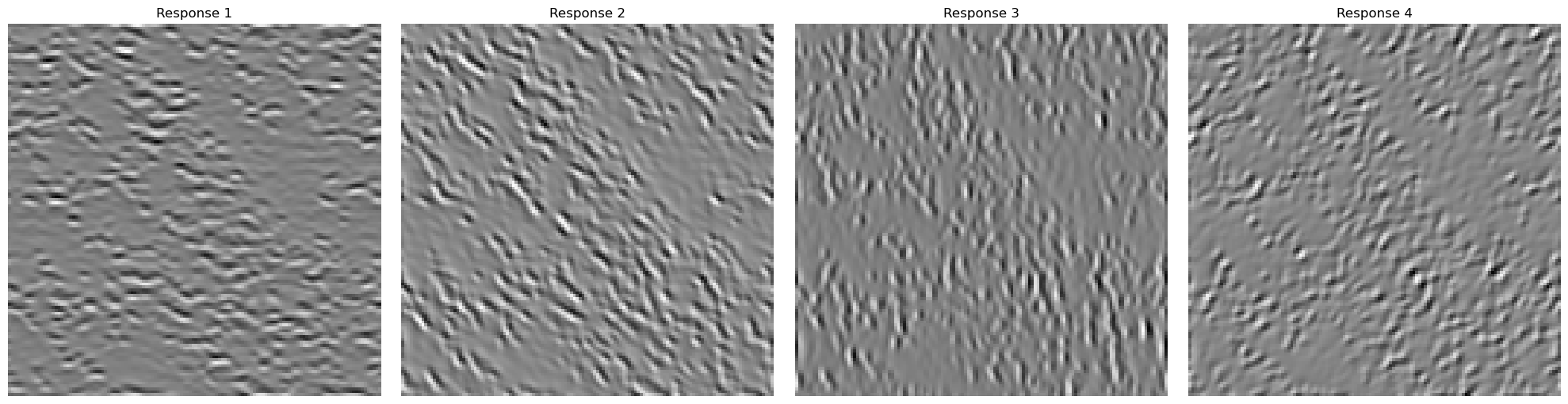
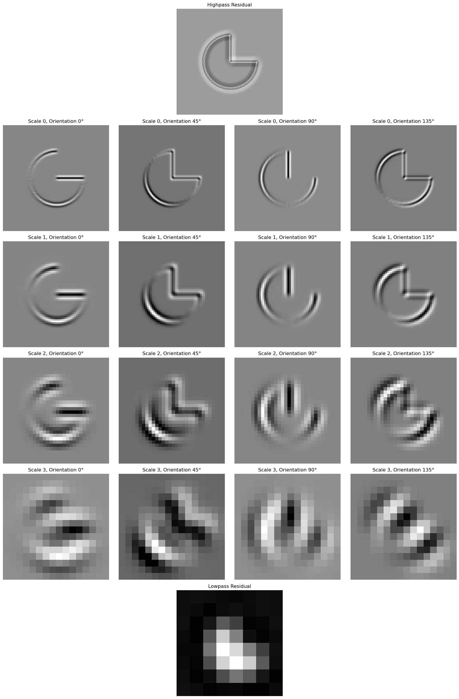
Each oriented filter will respond to certain edges and features at a specific orientation. With sp3_filters, we have 4 orientations (0°, 45°, 90°, 135°). The first orientation filter at 0° will highlight the changes in the y direction and so it will highlight the horizontal components of the edges in an image. Similarly, the 90° orientation filter will highlight the changes in the x direction and so it will highlight the vertical component of the edges in an image. The filters are called steerable because any linear combination of these basis filters can create any orientation you want. The sum of all oriented filters for a given band is the same as a standard laplacian band pass. Each of the filters are already by default bandpass filters because they each capture only a specific range of frequencies. When you sum all the orientation filters together, they form a circular band because they each capture different angles in a circle. In the frequency space, this is what a Laplacian band pass filter looks like. Here are some sample images convolved with each of the oriented filters and the combined response magnitude image which preserves all the components at different orientations.
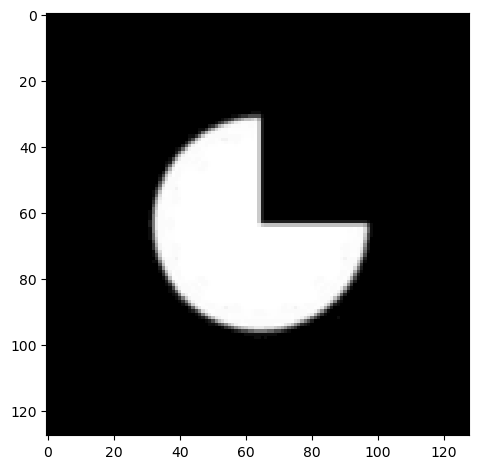


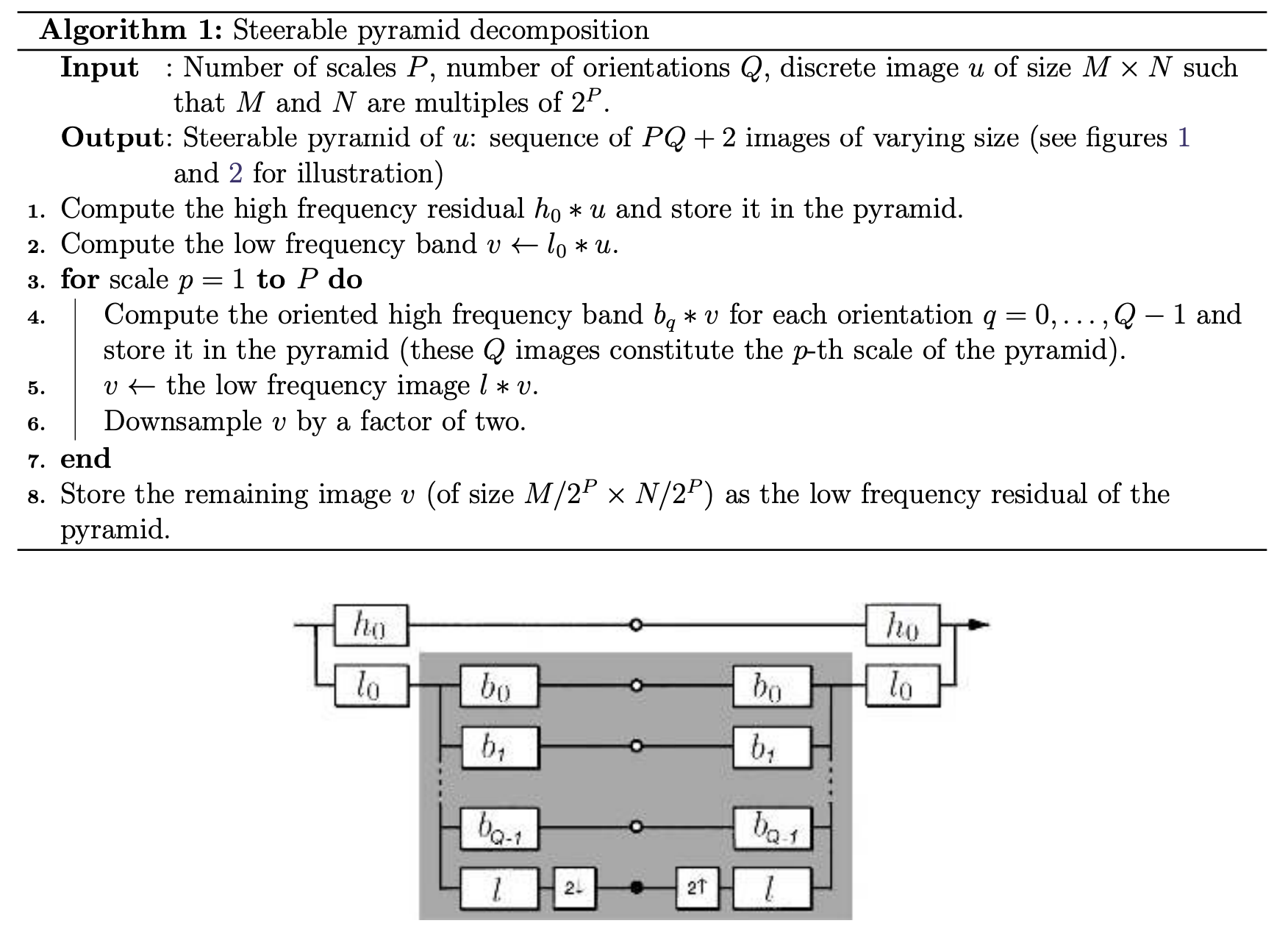
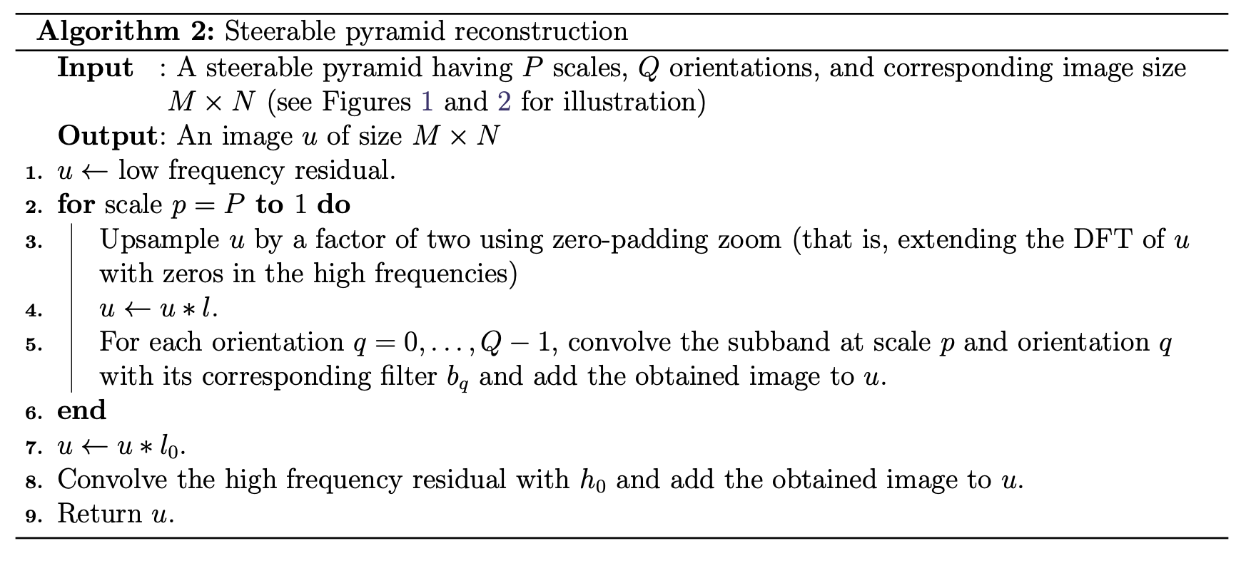
Once I got the aligned filters working, I implemented the oriented pyramid. This should be similar to the laplacian pyramid, and I essentially follow the paper's diagram for how to construct it. I start with one laplace layer, and on the low frequency component, I recurse with the oriented pyramid. Here is a sample image that I reconstructed using the oriented pyramid. After that, I use the pacman image to demonstrate that each of my orientations correspond to different oriented frequencies.
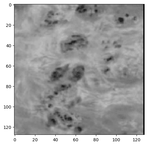
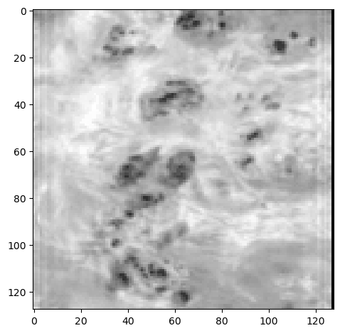
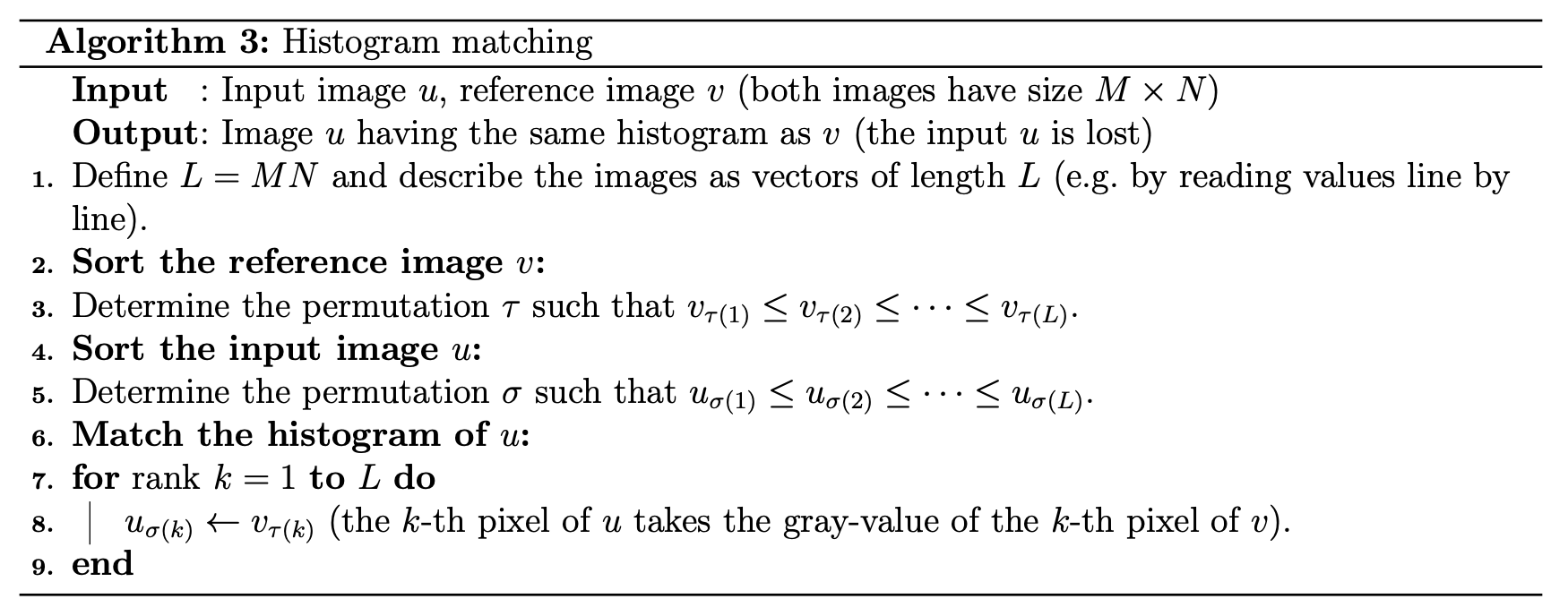
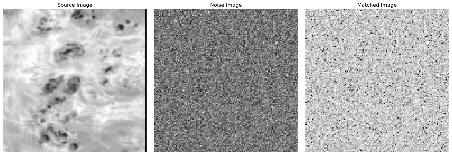
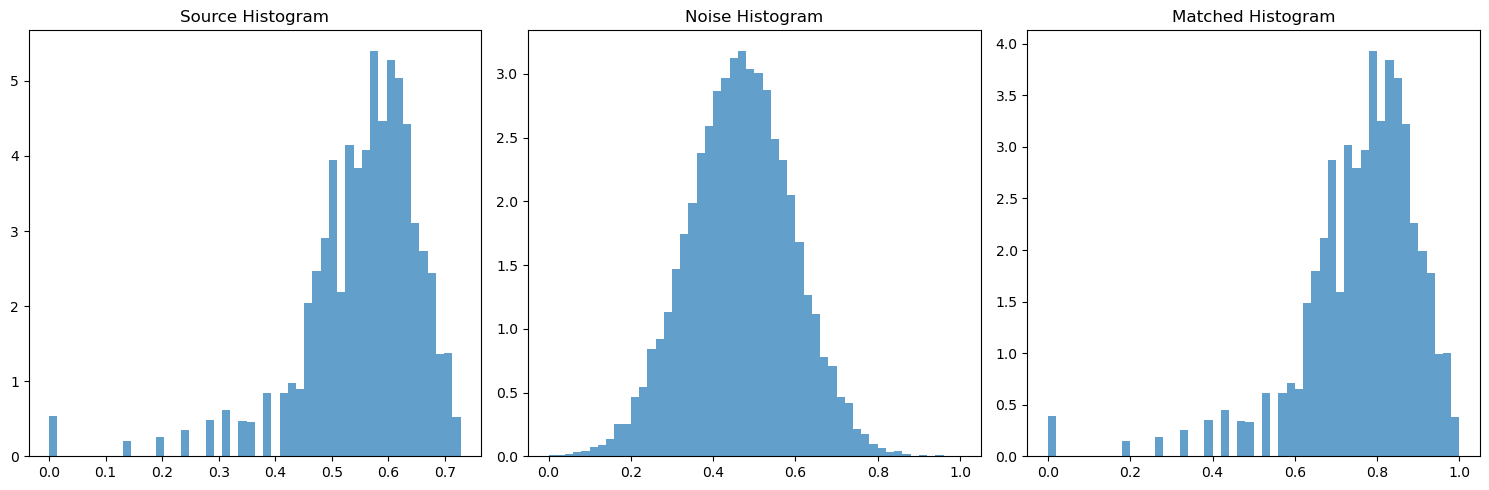
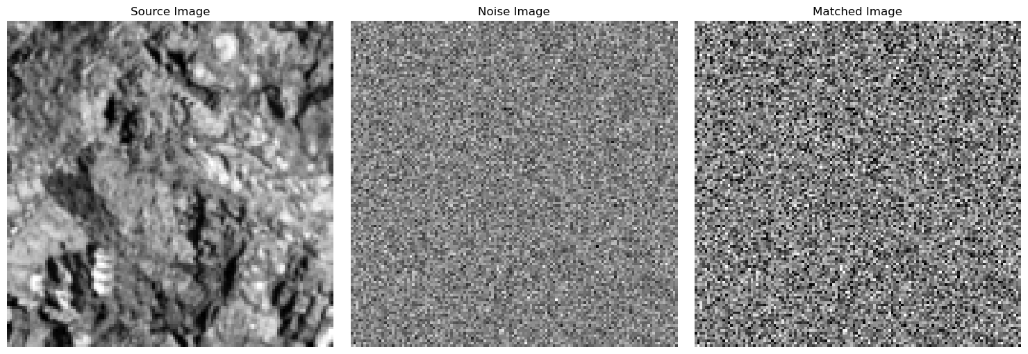
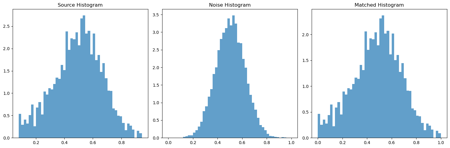
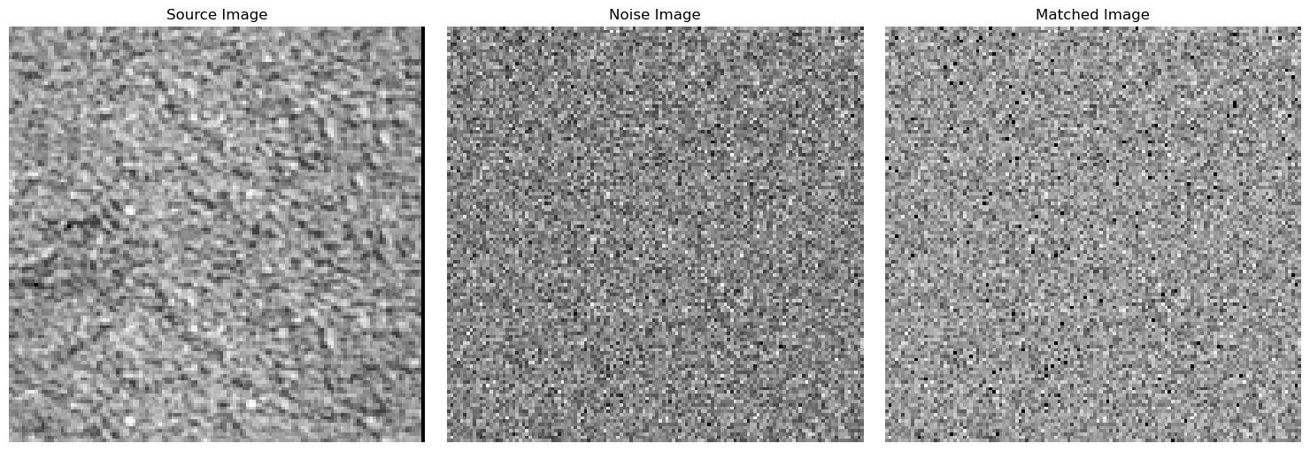
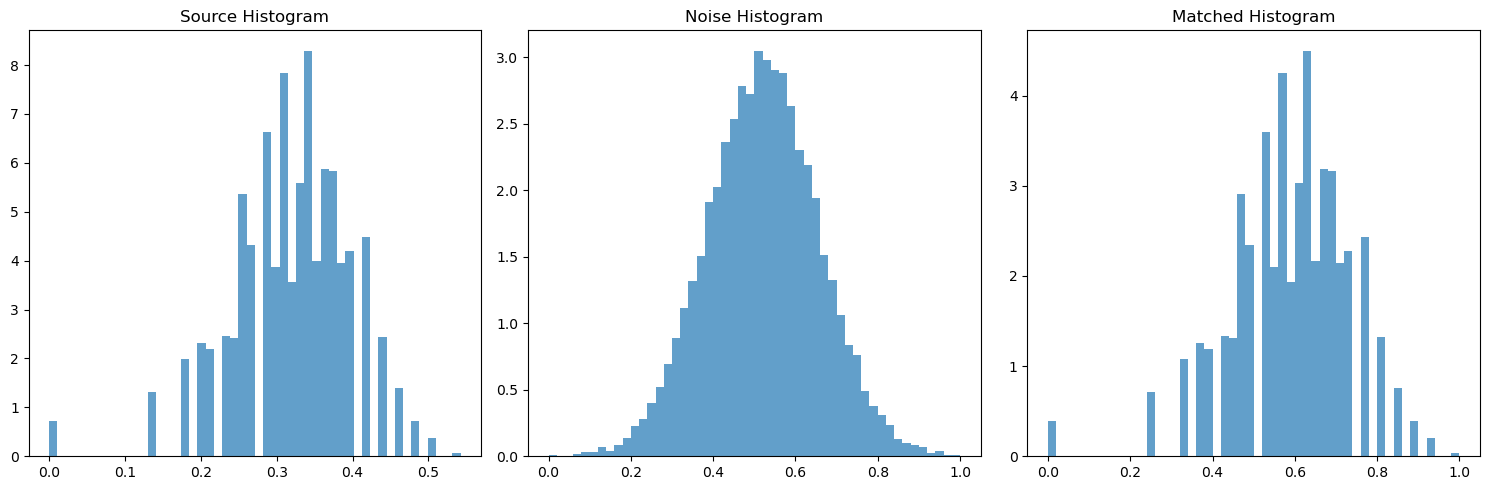
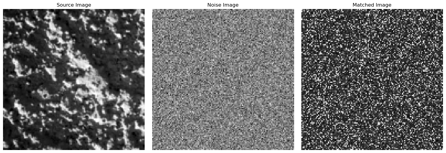
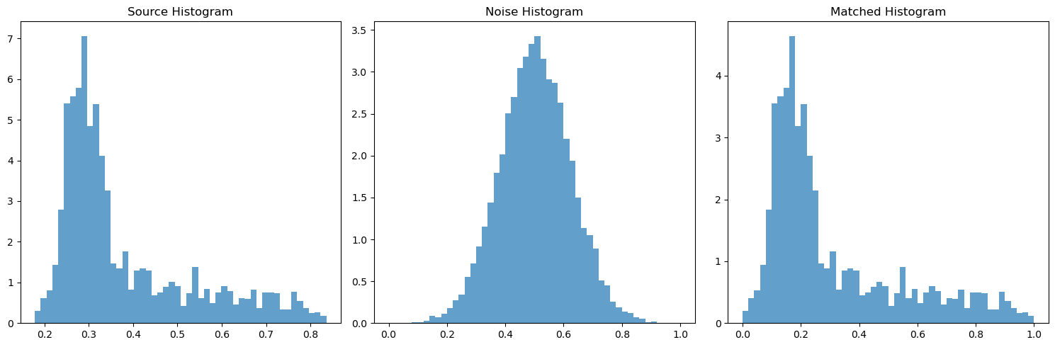
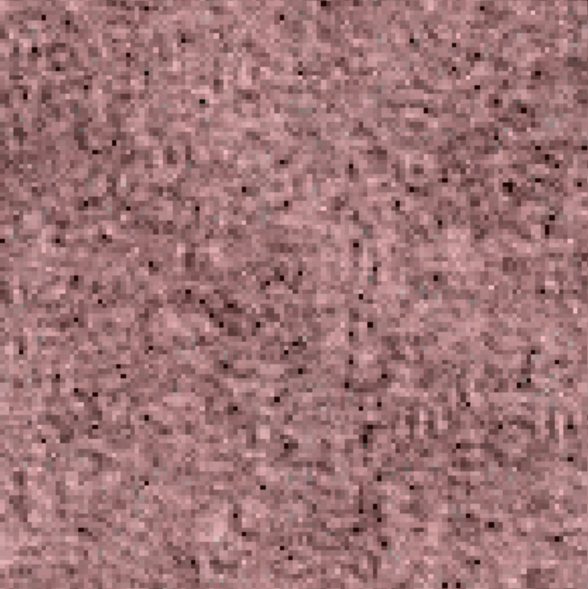
With the actual pyramid working, I needed to implement the histogram matching, which is named match-histogram in the paper and is outlined in pseudocode. Because this is all cumulative, I first made sure to unit test this code and all my code before. I had to make sure the histogram for some randomly initialized gaussian noise ends up matching the histogram of some source image. Below I have chosen some sample images and demonstrated that the histogram of the noisy image matches the histogram of the source image.
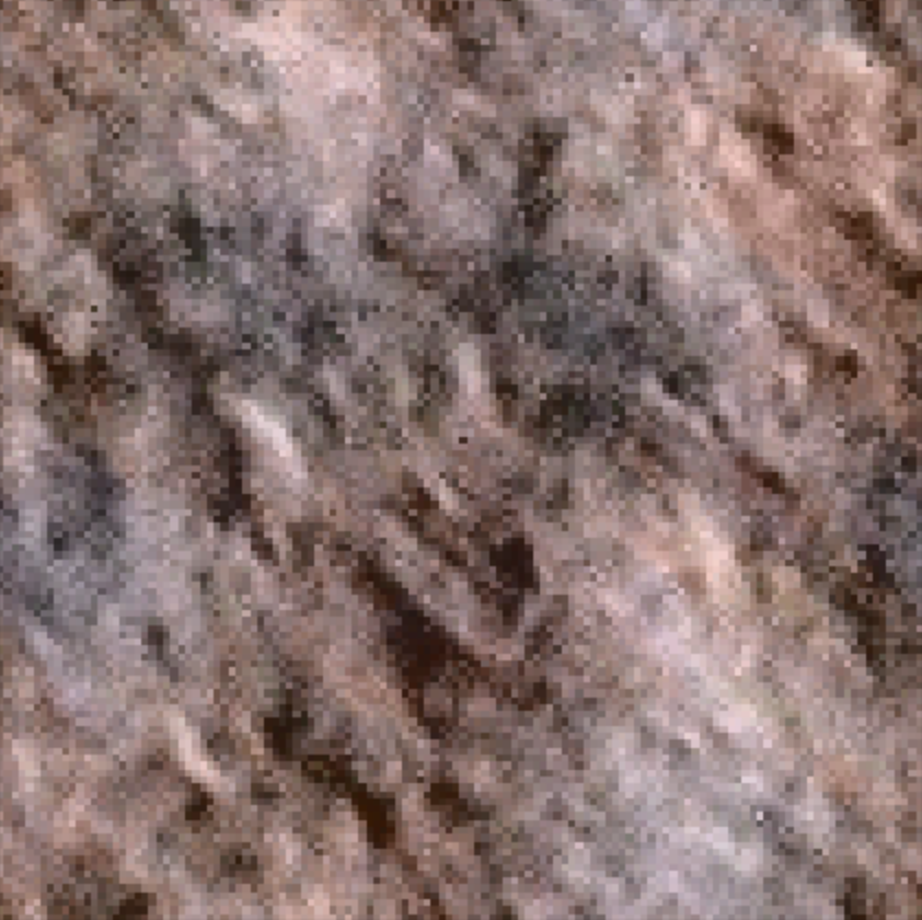
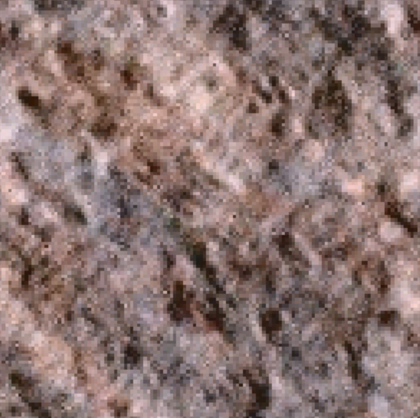
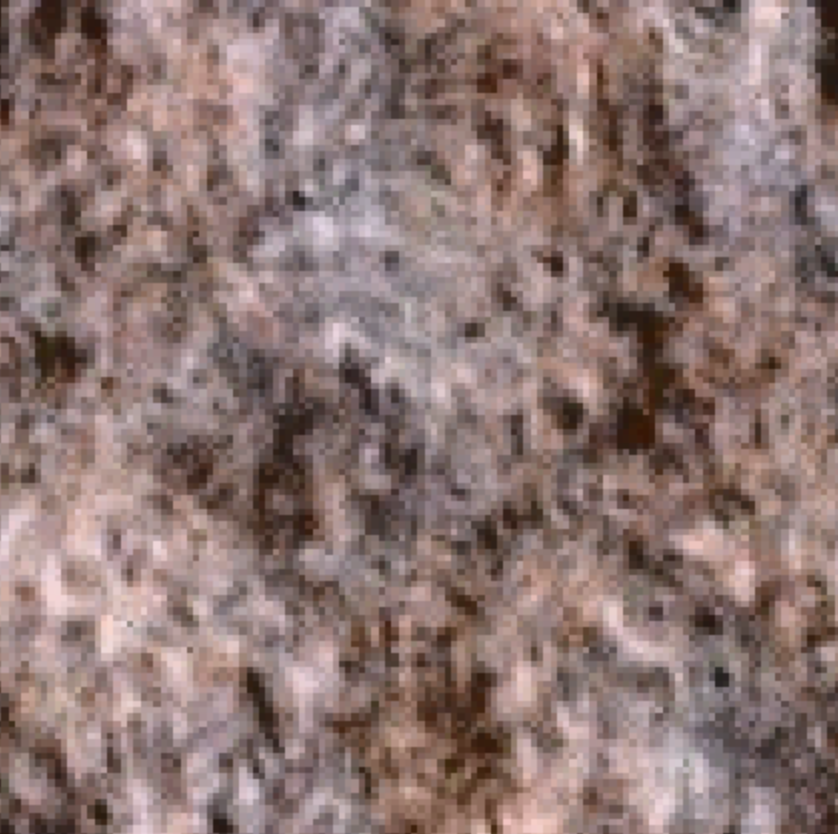
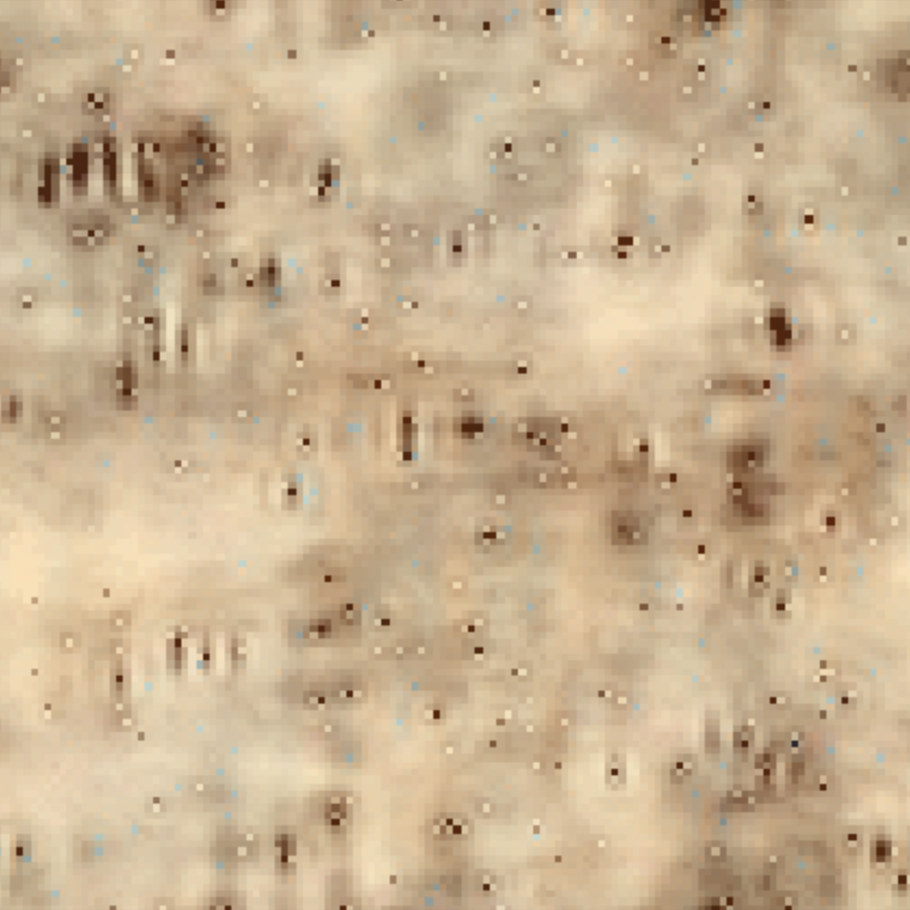
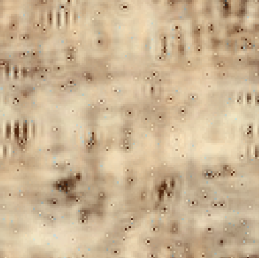
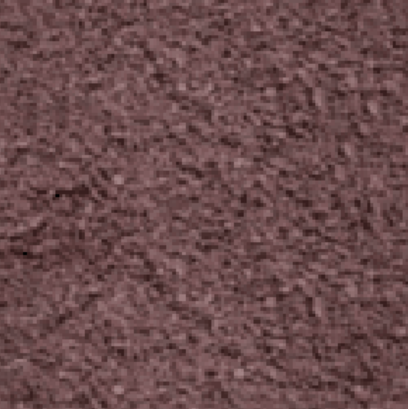
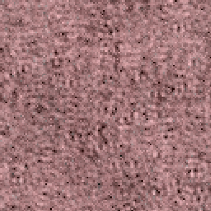
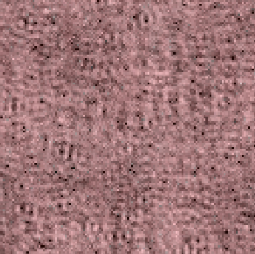
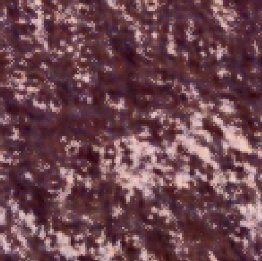
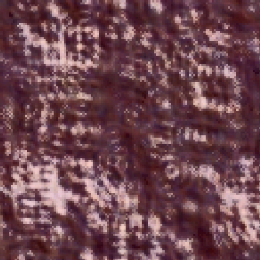
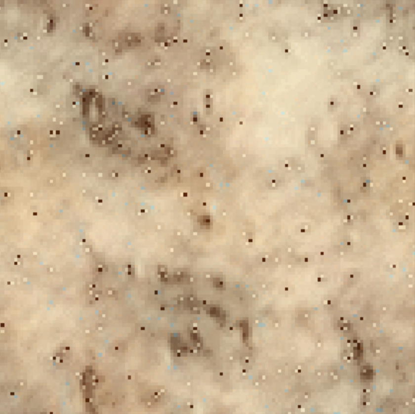
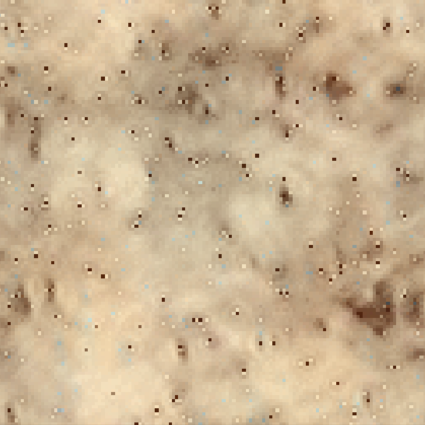
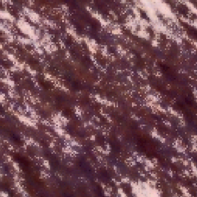
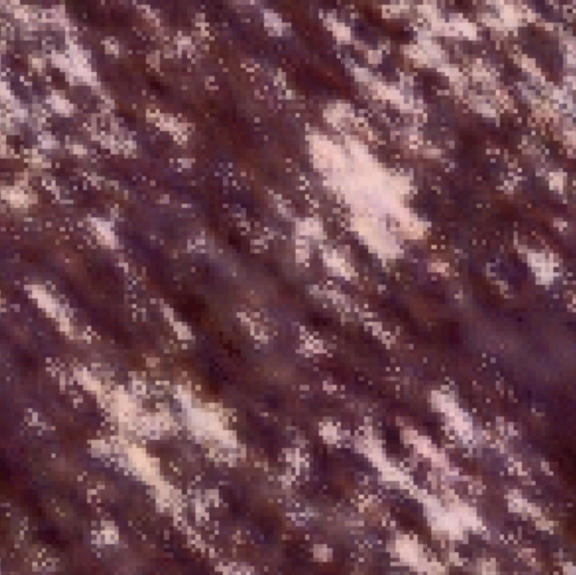
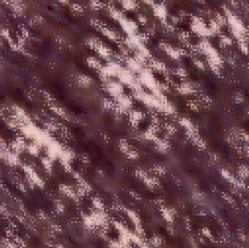
Finally, I implemented the texture synthesis algorithm, which is also outlined in pseudocode, named match-texture. This required me to use all the code I've implemented up until now. However, some extra considerations were needed to make this work. I needed to use wrap padding when convolving, and color images need to be dealt with properly. As described in the paper, for color images, I need to transform the 3-dimensional pixel values (RGB) of my source image into a PCA basis in order to de-correlate and normalize the pixel values. This enables me to operate on the RGB channels independently. For extra reading into practical considerations and greater detail on pseudocode and other misc, see this link here (https://www.ipol.im/pub/art/2014/79/article_lr.pdf), but this shouldn't be required to get the basic code running. The Heeger-Bergen texture synthesis algorithm for RGB color textures starts by first computing the PCA color space of the input texture. We do this because PCA considers color correlations and doesn't affect any spatial correlations. Then, we determine the channels of the input image in the PCA color space. Next, we apply the texture synthesis algorithm (Algorithm 4) on each PCA channel. This gives an output texture in the PCA color space. Therefore, the last step is to convert the output image into the RGB color space. The obtained RGB image is the output of the algorithm.

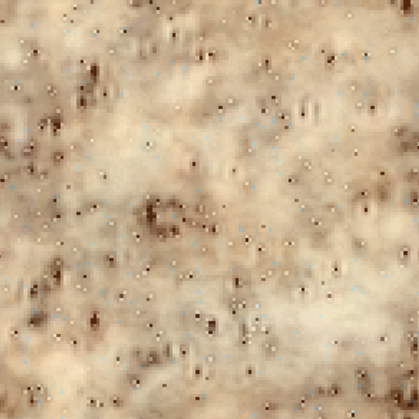
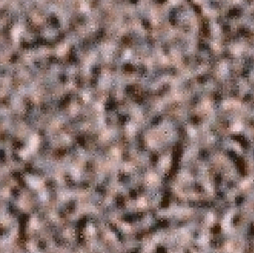
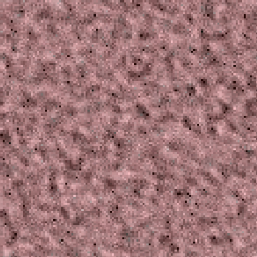
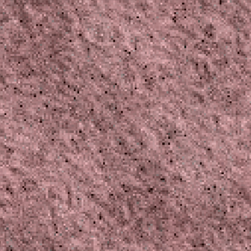
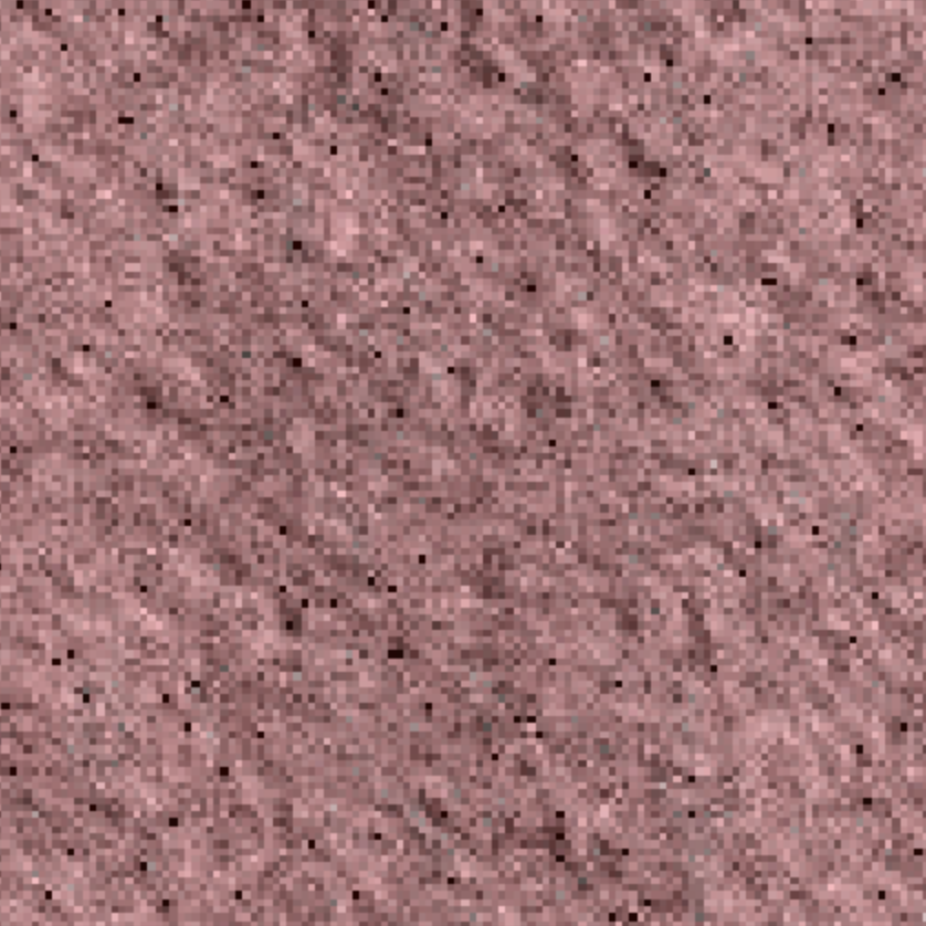
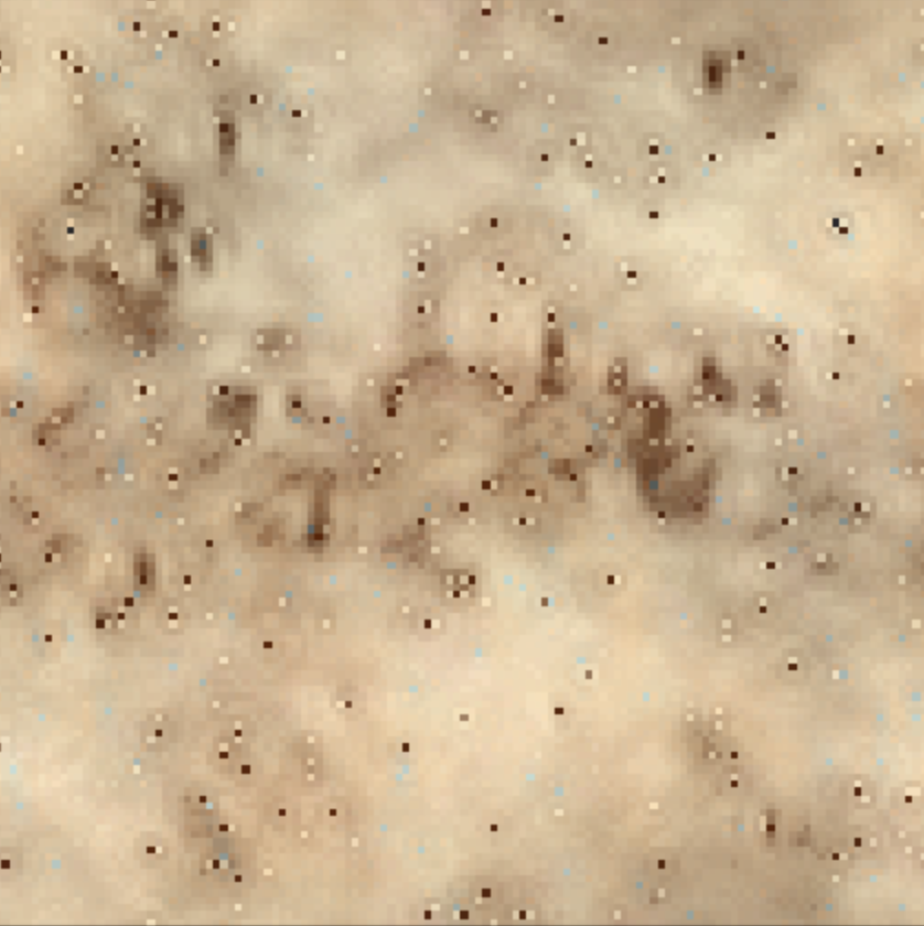
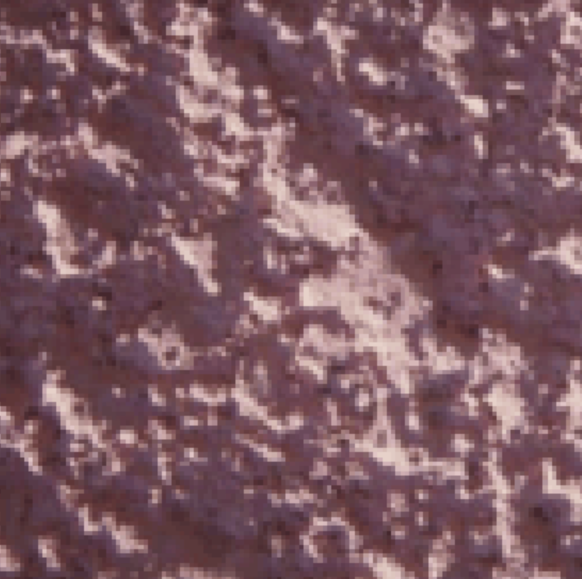
My algorithm didn't work so well on this image because it produces many small black dots and artifacts. This could possibly be due to not reconstructing the image correctly from the pyramid. Maybe using more orientation filters or increasing the number of scales would reduce the appearance of these artifacts.


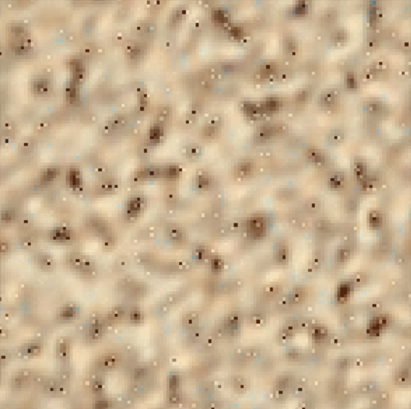
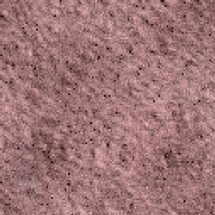
I made several design choices: operating in the spatial domain instead of the frequency domain, the kind of padding we used, the number of iterations, the number of oriented filters, etc. so I decided to ablate some of these and compare their performance.
Increasing the number of iterations improves the output texture but too many iterations makes the texture seem like it has a regular pattern on top of the existing original texture, as can be seen by iteration 20. After multiple experimentations, I found that by around the 4th and 5th iterations, the output is most similar to the original texture. There are no noticeable differences in the output texture for very large numbers of iterations past 20.

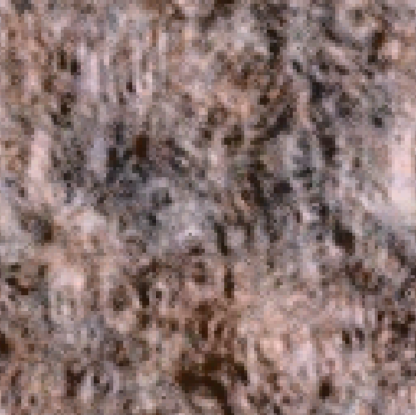

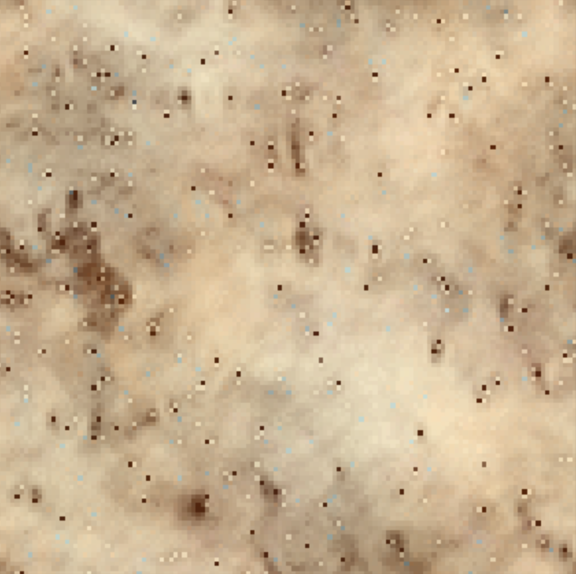
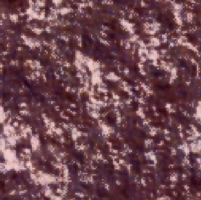
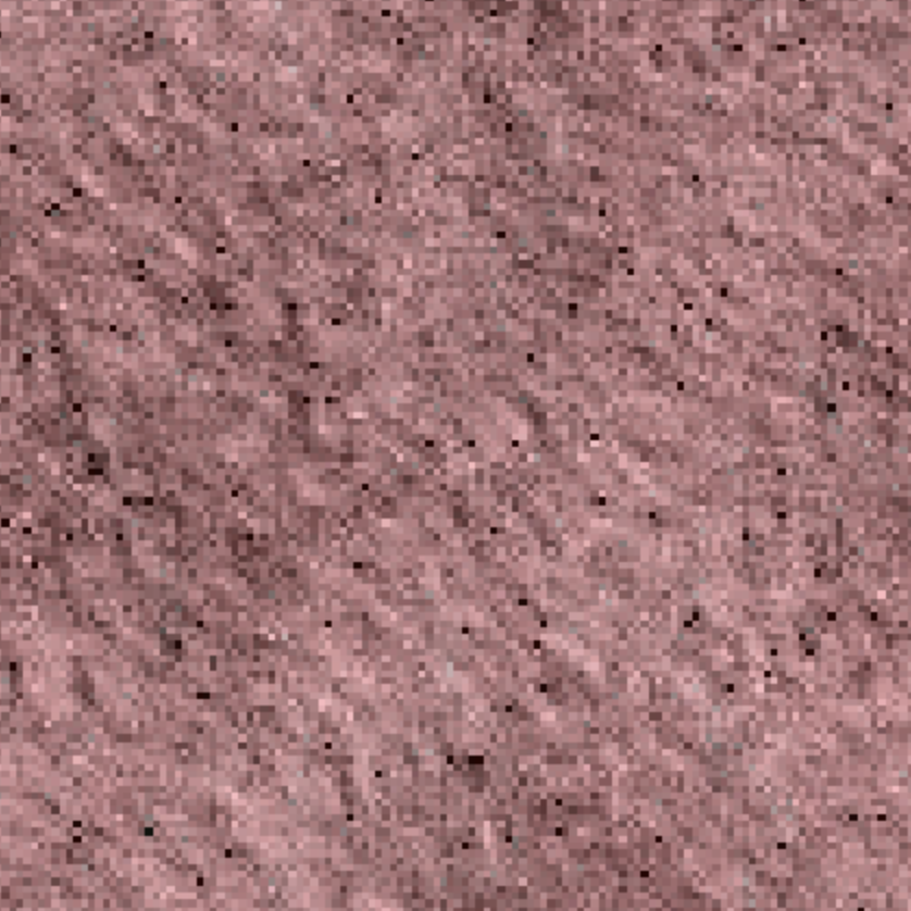
After I increased the number of orientation filters, the results improved for each iteration as the images looked more similar to the original texture. For textures that have no dominant orientation such as Texture 3, there seems to be no effect in changing the number of orientation filters. Furthermore, since more angles are captured if we use more orientation filters, the images look smoother maybe because there seems to be more overlap between the filters.


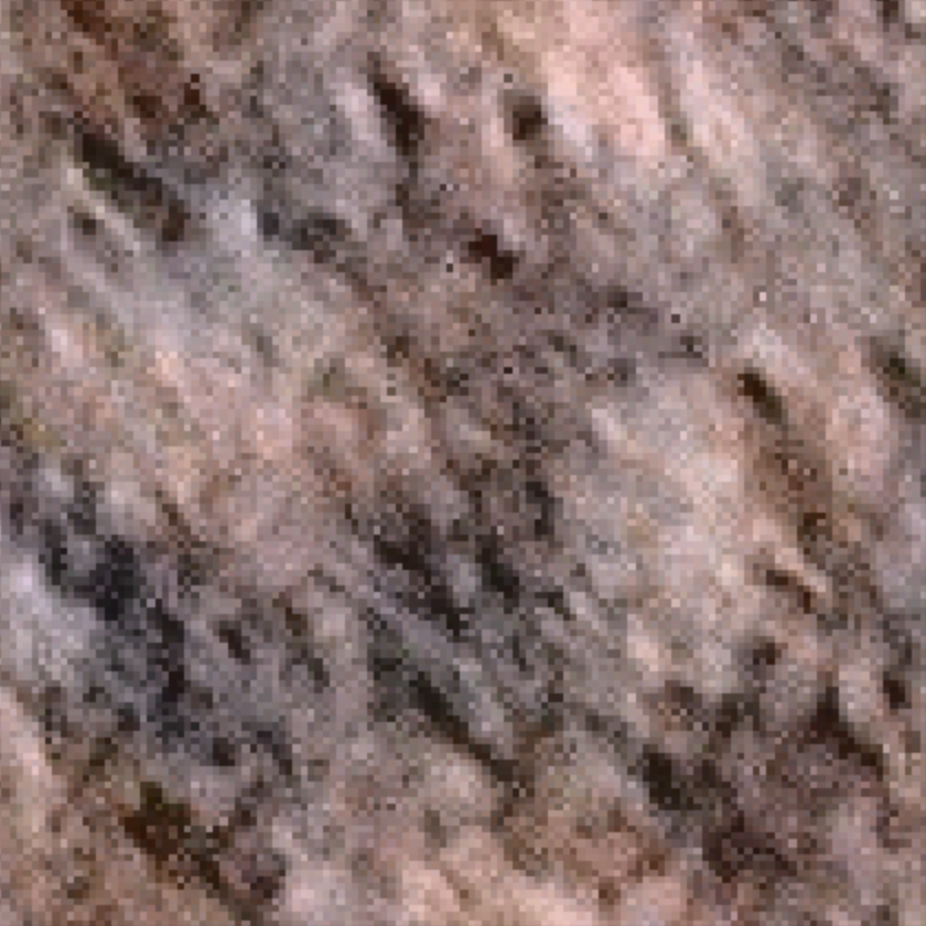
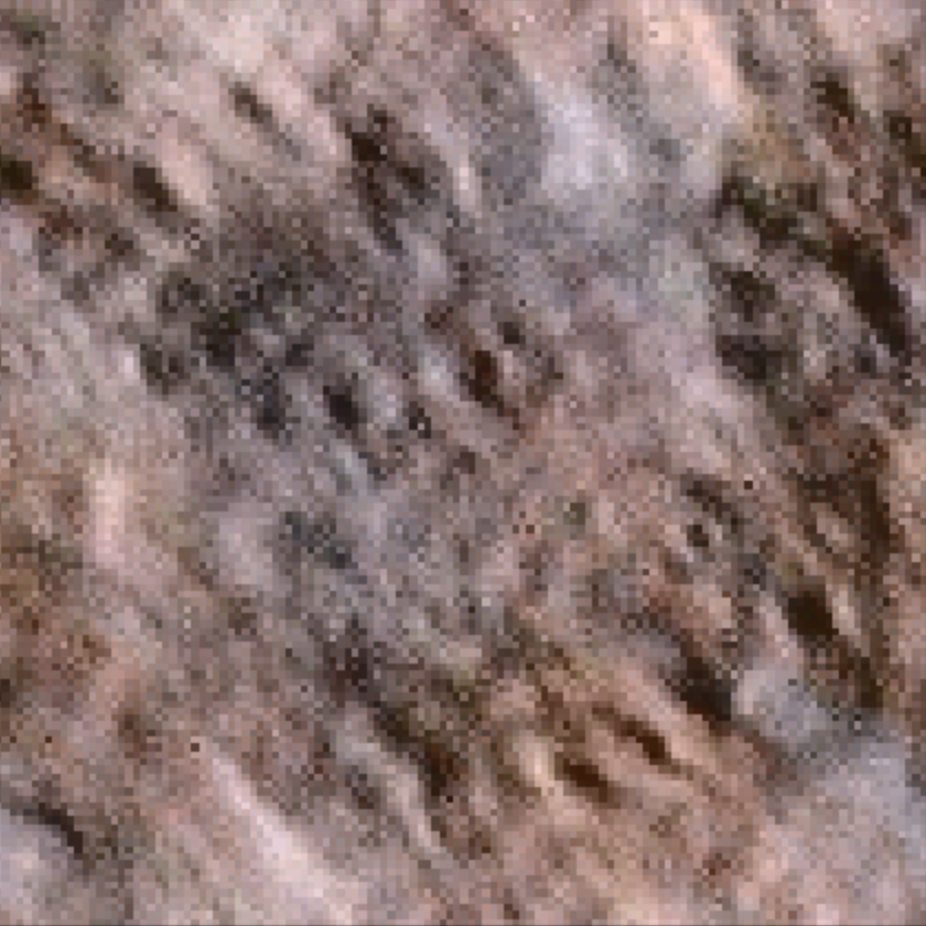
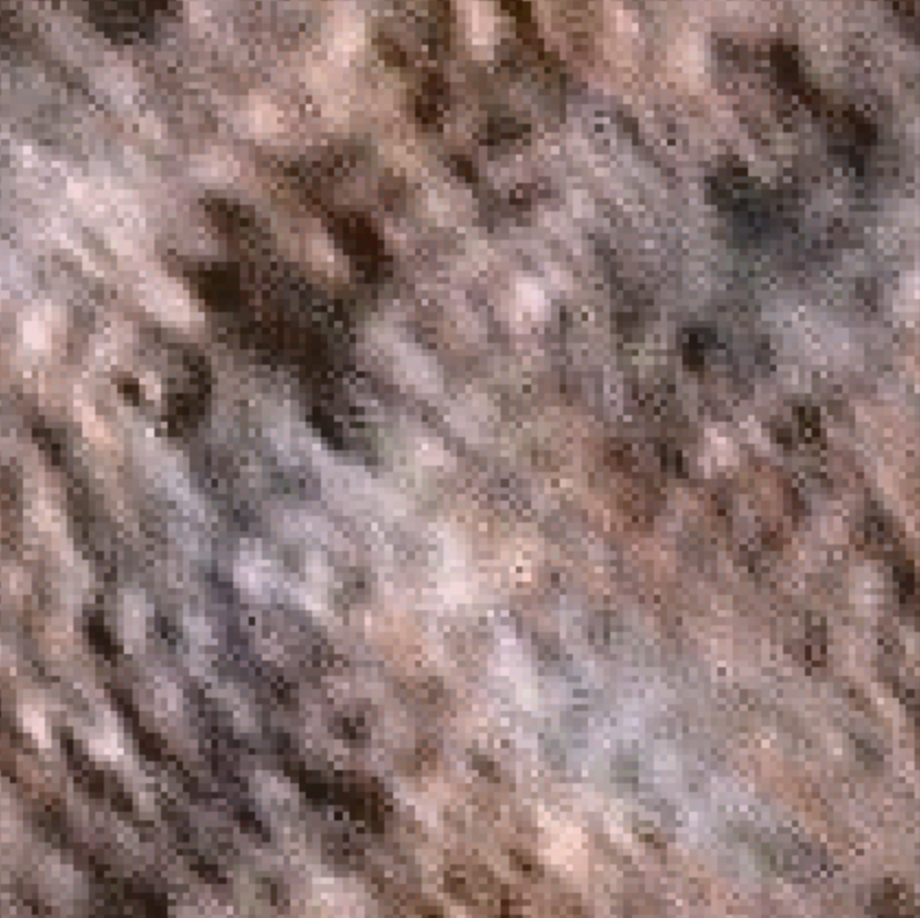

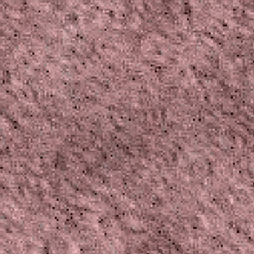
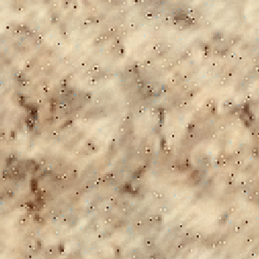
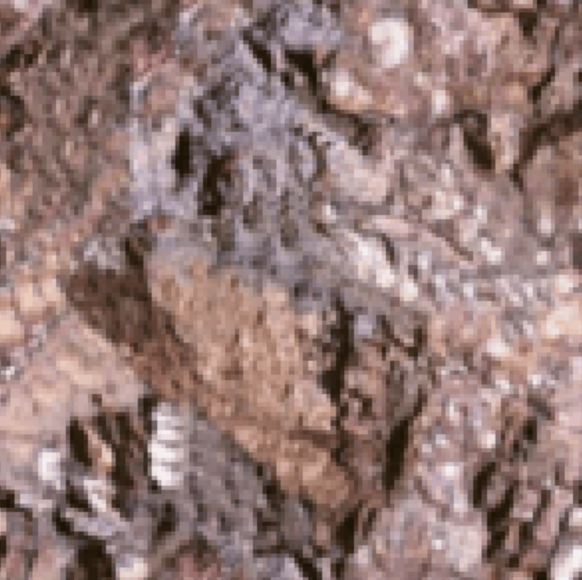
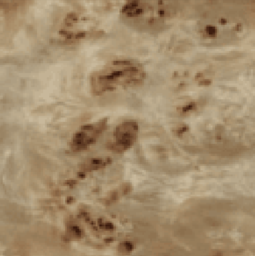
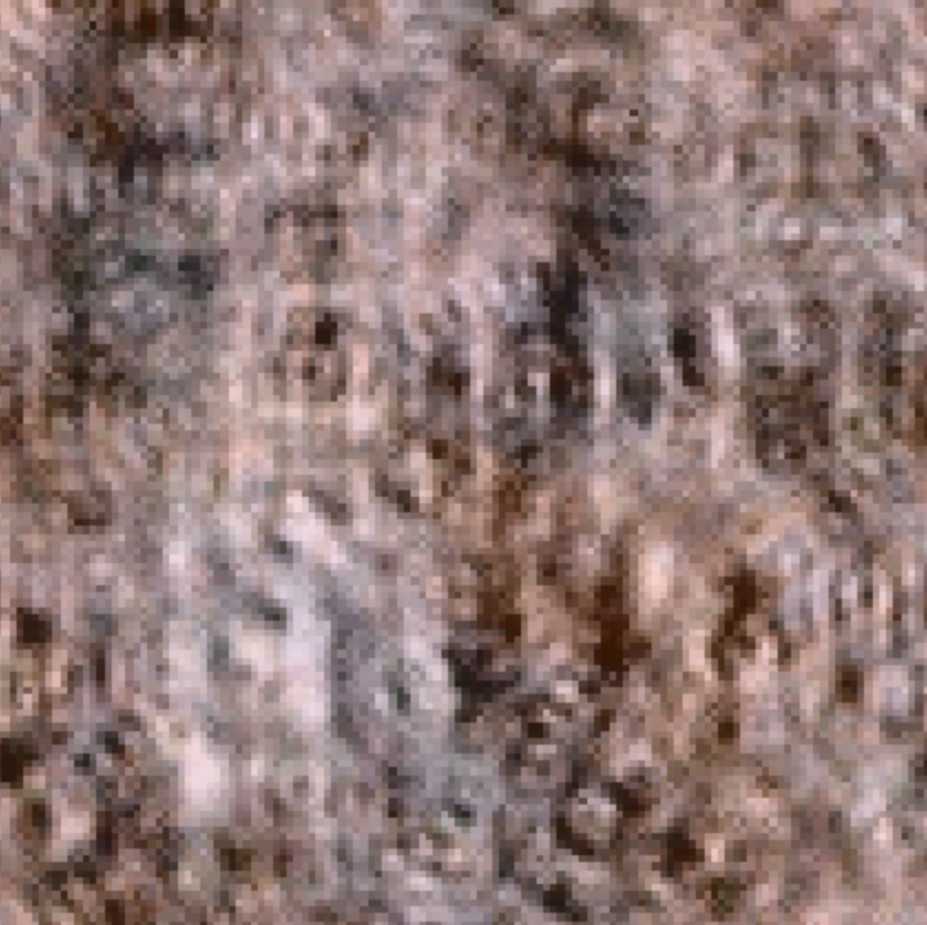
Varying the number of scales was by far the hyperparamater that had the most significant effect on the output texture. Increasing the number of scales improved the results as they looked more closely like the input textures. It removed the blotchy effect that you see in the images where the number of scales = 1. However, for textures like Texture 3 where there is no clear pattern, increasing the number of scales doesn't seem to affect it as much as textures where you can see more varied structures. Increasing the scales to the maximum possible allows us to capture all the details of the original input image which results in a better output texture.